Machine Learning for hackers读书笔记(十二)模型比较

标签：

library(‘ggplot2‘)
df <- read.csv(‘G:\\dataguru\\ML_for_Hackers\\ML_for_Hackers-master\\12-Model_Comparison\\data\\df.csv‘)

#用glm

logit.fit <- glm(Label ~ X + Y,family = binomial(link = ‘logit‘),data = df)

logit.predictions <- ifelse(predict(logit.fit) > 0, 1, 0)

mean(with(df, logit.predictions == Label))
#正确率 0.5156,跟猜差不多一样的结果

library(‘e1071‘) 

svm.fit <- svm(Label ~ X + Y, data = df)

svm.predictions <- ifelse(predict(svm.fit) > 0, 1, 0)

mean(with(df, svm.predictions == Label))

#改用SVM,正确率72%

library("reshape")

#df中的字段,X,Y,Label,Logit,SVM

df <- cbind(df,data.frame(Logit = ifelse(predict(logit.fit) > 0, 1, 0),SVM = ifelse(predict(svm.fit) > 0, 1, 0))) 

#melt的结果,增加字段variable,其中的值有Label,Logit,SVM,增加字段value,根据variable取相应的值

#melt函数:指定变量,将其他剩下的字段作为一个列,把对应的取值列出.melt和cast,好像是相反的功能

predictions <- melt(df, id.vars = c(‘X‘, ‘Y‘)) 

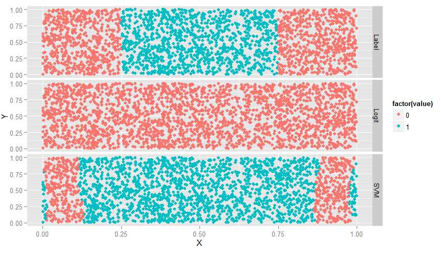
ggplot(predictions, aes(x = X, y = Y, color = factor(value))) +  geom_point() +  facet_grid(variable ~ .)

#如下图,Label为真实结果,Lgm完全没用,而SVM有所识别,但边缘不对

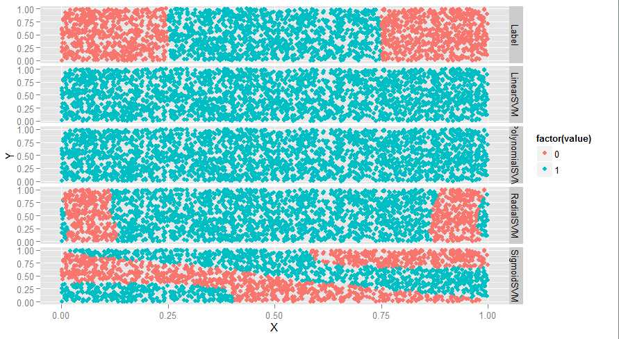
#SVM函数有个kernel参数,取值有4个:linear,polynomial,radial和sigmoid,4个都画出来看看

df <- df[, c(‘X‘, ‘Y‘, ‘Label‘)] 

linear.svm.fit <- svm(Label ~ X + Y, data = df, kernel = ‘linear‘)

with(df, mean(Label == ifelse(predict(linear.svm.fit) > 0, 1, 0))) 

polynomial.svm.fit <- svm(Label ~ X + Y, data = df, kernel = ‘polynomial‘)

with(df, mean(Label == ifelse(predict(polynomial.svm.fit) > 0, 1, 0))) 

radial.svm.fit <- svm(Label ~ X + Y, data = df, kernel = ‘radial‘)

with(df, mean(Label == ifelse(predict(radial.svm.fit) > 0, 1, 0))) 

sigmoid.svm.fit <- svm(Label ~ X + Y, data = df, kernel = ‘sigmoid‘)

with(df, mean(Label == ifelse(predict(sigmoid.svm.fit) > 0, 1, 0))) 

df <- cbind(df,

            data.frame(LinearSVM = ifelse(predict(linear.svm.fit) > 0, 1, 0),

                       PolynomialSVM = ifelse(predict(polynomial.svm.fit) > 0, 1, 0),

                       RadialSVM = ifelse(predict(radial.svm.fit) > 0, 1, 0),

                       SigmoidSVM = ifelse(predict(sigmoid.svm.fit) > 0, 1, 0))) 

predictions <- melt(df, id.vars = c(‘X‘, ‘Y‘)) 

ggplot(predictions, aes(x = X, y = Y, color = factor(value))) +  geom_point() +  facet_grid(variable ~ .)

#如下图,线性和多项式没用,radial还行,sigmoid很奇怪

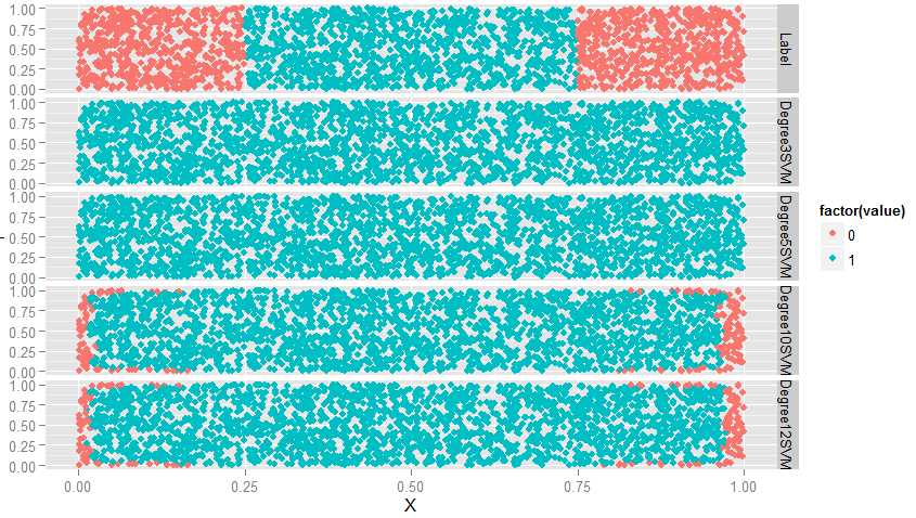
#svm有个参数叫degree,看看效果

polynomial.degree3.svm.fit <- svm(Label ~ X + Y, data = df, kernel = ‘polynomial‘, degree = 3)

with(df, mean(Label != ifelse(predict(polynomial.degree3.svm.fit) > 0, 1, 0))) 

polynomial.degree5.svm.fit <- svm(Label ~ X + Y,data = df,kernel = ‘polynomial‘,degree = 5)

with(df, mean(Label != ifelse(predict(polynomial.degree5.svm.fit) > 0, 1, 0))) 

polynomial.degree10.svm.fit <- svm(Label ~ X + Y,data = df,kernel = ‘polynomial‘,degree = 10)

with(df, mean(Label != ifelse(predict(polynomial.degree10.svm.fit) > 0, 1, 0))) 

polynomial.degree12.svm.fit <- svm(Label ~ X + Y, data = df,  kernel = ‘polynomial‘,  degree = 12)

with(df, mean(Label != ifelse(predict(polynomial.degree12.svm.fit) > 0, 1, 0))) 

df <- df[, c(‘X‘, ‘Y‘, ‘Label‘)] 

df <- cbind(df,

            data.frame(Degree3SVM = ifelse(predict(polynomial.degree3.svm.fit) > 0,  1, 0),

                       Degree5SVM = ifelse(predict(polynomial.degree5.svm.fit) > 0, 1, 0),

                       Degree10SVM = ifelse(predict(polynomial.degree10.svm.fit) > 0, 1,  0),

                       Degree12SVM = ifelse(predict(polynomial.degree12.svm.fit) > 0,1, 0))) 

predictions <- melt(df, id.vars = c(‘X‘, ‘Y‘)) 

ggplot(predictions, aes(x = X, y = Y, color = factor(value))) +  geom_point() +  facet_grid(variable ~ .)

#从图上看,degreee提升,准确率也提升,此时会有过拟合问题,因此,当使用多项式核函数时,要对degree进行交叉验证

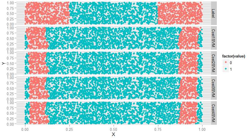
#接下来研究一下SVM的cost参数

radial.cost1.svm.fit <- svm(Label ~ X + Y, data = df,  kernel = ‘radial‘, cost = 1)

with(df, mean(Label == ifelse(predict(radial.cost1.svm.fit) > 0, 1, 0))) 

radial.cost2.svm.fit <- svm(Label ~ X + Y,  data = df,  kernel = ‘radial‘,  cost = 2)

with(df, mean(Label == ifelse(predict(radial.cost2.svm.fit) > 0, 1, 0))) 

radial.cost3.svm.fit <- svm(Label ~ X + Y,  data = df,   kernel = ‘radial‘,  cost = 3)

with(df, mean(Label == ifelse(predict(radial.cost3.svm.fit) > 0, 1, 0))) 

radial.cost4.svm.fit <- svm(Label ~ X + Y,  data = df,  kernel = ‘radial‘,  cost = 4)

with(df, mean(Label == ifelse(predict(radial.cost4.svm.fit) > 0, 1, 0))) 

df <- df[, c(‘X‘, ‘Y‘, ‘Label‘)] 

df <- cbind(df,

            data.frame(Cost1SVM = ifelse(predict(radial.cost1.svm.fit) > 0, 1, 0),

                       Cost2SVM = ifelse(predict(radial.cost2.svm.fit) > 0, 1, 0),

                       Cost3SVM = ifelse(predict(radial.cost3.svm.fit) > 0, 1, 0),

                       Cost4SVM = ifelse(predict(radial.cost4.svm.fit) > 0, 1, 0))) 

predictions <- melt(df, id.vars = c(‘X‘, ‘Y‘)) 

ggplot(predictions, aes(x = X, y = Y, color = factor(value))) +  geom_point() +  facet_grid(variable ~ .)

#如图,cost参数值提升使得效果越来越差,改变非常小,只能通过边缘数据察觉到效果越来越差

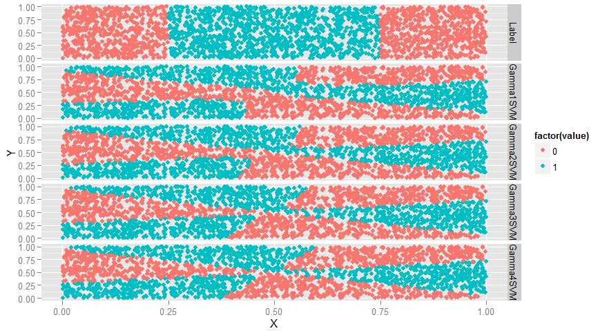
#再来看SVM的参数gamma

sigmoid.gamma1.svm.fit <- svm(Label ~ X + Y, data = df,   kernel = ‘sigmoid‘,  gamma = 1)

with(df, mean(Label == ifelse(predict(sigmoid.gamma1.svm.fit) > 0, 1, 0)))

sigmoid.gamma2.svm.fit <- svm(Label ~ X + Y, data = df,  kernel = ‘sigmoid‘, gamma = 2)

with(df, mean(Label == ifelse(predict(sigmoid.gamma2.svm.fit) > 0, 1, 0)))

sigmoid.gamma3.svm.fit <- svm(Label ~ X + Y, data = df, kernel = ‘sigmoid‘, gamma = 3)

with(df, mean(Label == ifelse(predict(sigmoid.gamma3.svm.fit) > 0, 1, 0))) 

sigmoid.gamma4.svm.fit <- svm(Label ~ X + Y,  data = df,   kernel = ‘sigmoid‘,   gamma = 4)

with(df, mean(Label == ifelse(predict(sigmoid.gamma4.svm.fit) > 0, 1, 0)))

df <- df[, c(‘X‘, ‘Y‘, ‘Label‘)] 

df <- cbind(df,

            data.frame(Gamma1SVM = ifelse(predict(sigmoid.gamma1.svm.fit) > 0, 1, 0),

                       Gamma2SVM = ifelse(predict(sigmoid.gamma2.svm.fit) > 0, 1, 0),

                       Gamma3SVM = ifelse(predict(sigmoid.gamma3.svm.fit) > 0, 1, 0),

                       Gamma4SVM = ifelse(predict(sigmoid.gamma4.svm.fit) > 0, 1, 0))) 

predictions <- melt(df, id.vars = c(‘X‘, ‘Y‘)) 

ggplot(predictions, aes(x = X, y = Y, color = factor(value))) +  geom_point() +  facet_grid(variable ~ .)

#变弯曲了

 #SVM介绍完毕,意思就是碰到数据集要调参,下面比较一下SVM,glm和KNN的表现

load(‘G:\\dataguru\\ML_for_Hackers\\ML_for_Hackers-master\\12-Model_Comparison\\data\\dtm.RData‘)

set.seed(1) 

#一半训练,一半测试

training.indices <- sort(sample(1:nrow(dtm), round(0.5 * nrow(dtm))))

test.indices <- which(! 1:nrow(dtm) %in% training.indices) 

train.x <- dtm[training.indices, 3:ncol(dtm)]

train.y <- dtm[training.indices, 1] 

test.x <- dtm[test.indices, 3:ncol(dtm)]

test.y <- dtm[test.indices, 1] 

rm(dtm) 

library(‘glmnet‘)

regularized.logit.fit <- glmnet(train.x, train.y, family = c(‘binomial‘)) 

lambdas <- regularized.logit.fit$lambda 

performance <- data.frame() 

for (lambda in lambdas)

{

  predictions <- predict(regularized.logit.fit, test.x, s = lambda)

  predictions <- as.numeric(predictions > 0)

  mse <- mean(predictions != test.y)

  performance <- rbind(performance, data.frame(Lambda = lambda, MSE = mse))

} 

ggplot(performance, aes(x = Lambda, y = MSE)) +  geom_point() +  scale_x_log10()

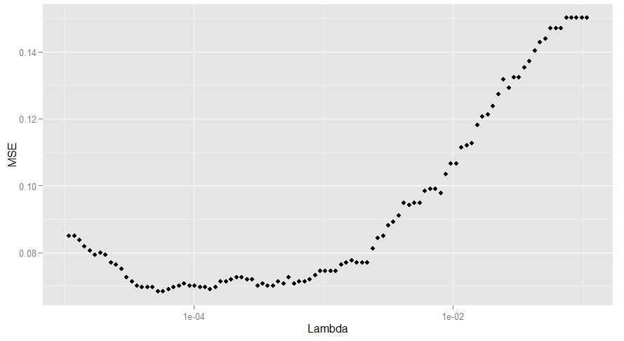
#有两个lambda对应的错误率是最小的,我们选了较大的那个,因为这意味着更强的正则化

best.lambda <- with(performance, max(Lambda[which(MSE == min(MSE))])) 

#算一下mse,0.068

mse <- with(subset(performance, Lambda == best.lambda), MSE)

#下面试一下SVM

library(‘e1071‘)

#这一步时间很长,因为数据集大,进行线性核函数时间长

linear.svm.fit <- svm(train.x, train.y, kernel = ‘linear‘) 

predictions <- predict(linear.svm.fit, test.x)

predictions <- as.numeric(predictions > 0) 

mse <- mean(predictions != test.y) 

mse

#0.128,错误率12%,比glm还高.为了达到最优效果,应该尝试不同的cost超参数

radial.svm.fit <- svm(train.x, train.y, kernel = ‘radial‘)

predictions <- predict(radial.svm.fit, test.x)

predictions <- as.numeric(predictions > 0) 

mse <- mean(predictions != test.y) 

mse

#错误率,0.1421538,比刚才还高,因此知道径向核函数效果不好,那么可能边界是线性的.所以glm效果才会比较好.

#下面试一下KNN,KNN对于非线性效果好

library(‘class‘) 

knn.fit <- knn(train.x, test.x, train.y, k = 50) 

predictions <- as.numeric(as.character(knn.fit)) 

mse <- mean(predictions != test.y) 

mse

#错误率0.1396923,说明真的有可能是线性模型,下面试一下哪个K效果最好

performance <- data.frame() 

for (k in seq(5, 50, by = 5))

{

  knn.fit <- knn(train.x, test.x, train.y, k = k)

  predictions <- as.numeric(as.character(knn.fit))

  mse <- mean(predictions != test.y)

  performance <- rbind(performance, data.frame(K = k, MSE = mse))

} 

best.k <- with(performance, K[which(MSE == min(MSE))]) 

best.mse <- with(subset(performance, K == best.k), MSE) 

best.mse

#错误率降到0.09169231,KNN效果介于glm和SVM之间

#因此,最优选择是glm

Machine Learning for hackers读书笔记(十二)模型比较

标签：

原文地址：http://www.cnblogs.com/MarsMercury/p/4964885.html