在本练习中,先介绍了SVM的一些基本知识,再使用SVM(支持向量机 )实现一个垃圾邮件分类器。
在开始之前,先简单介绍一下SVM
①从逻辑回归的 cost function 到SVM 的 cost function
逻辑回归的假设函数如下:
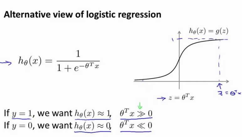
hθ(x)取值范围为[0,1],约定hθ(x)>=0.5,也即θT·x >=0时,y=1;比如hθ(x)=0.6,此时表示有60%的概率相信 y 等于1
显然,要想让y取值为1,hθ(x)越大越好,因为hθ(x)越大,y 取值为1的概率也就越大,也即:更好把握相信 y 等于1。而要想hθ(x)越大,也就是θT·x远远大于0
The larger θT·x is, the larger also is hθ(x) = p(y = 1|x; w, b), and thus also the higher our degree of “confidence”
that the label is 1
同理,y 等于0,也可以通过类似的推理得到:要想让 y 取值为0,则hθ(x)越小越好,而要想hθ(x)越小,也就是θT·x远远小于0
逻辑回归的代价函数(cost function)如下:(为了方便讨论,假设 training examples 只有一个,即:m = 1)
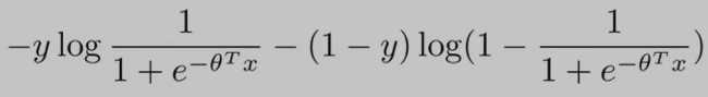
从上面的cost function公式 可以看出:当y==0时,只有右边的那部分式子起作用;当y==1时,(1-y==0)只有左边的那部分式子起作用。
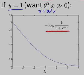
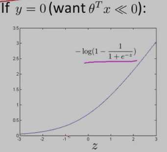
y==1时,逻辑回归的代价函数的图形表示如下:可以看出,逻辑回归的代价函数在整个坐标轴上是连续的。
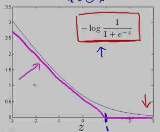
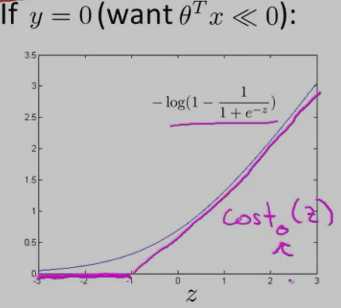
在上面的y==1时的逻辑回归代价函数的基础上,构造一条新的代价函数曲线,记为cost1(z) ,(用紫色的两条直线 线段表示,z==1处是转折点),如下图:在z==1 点,新的代价函数是不连续的。
同理,y==0时,逻辑回归的代价函数的图形表示如下图:可以看出,逻辑回归的代价函数在整个坐标轴上是连续的。
在上面的y==0时的逻辑回归代价函数的基础上,构造一条新的代价函数曲线,记为cost0(z)(用紫色的两条直线 线段表示,z== -1处是转折点),如下图:在z== -1 点,新的代价函数是不连续的。
使用上面新构造的两条函数曲线:cost0(z) 和 cost1(z) (z 等于θT·x),组成了支持向量机(SVM)的cost function,如下:
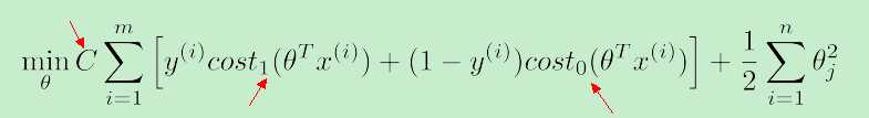
对于training example的数目 m 而言,它是一个常量,故在SVM的cost function中 去掉了 m
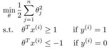
因此,总结一下,得到SVM的代价函数如下:
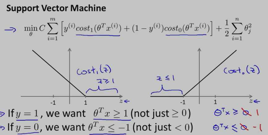
对于SVM而言,y==1时,要求:θT·x>=1;y==0时,要求:θT·x<=-1
可以看出:相比于逻辑回归,SVM中的 label of result y 等于 1 时,要求θT·x大于等于1,而不是0,这就相当于多了提高了限制条件,多了一层保障。
另外,SVM的代价函数中的 参数 C 就相当于逻辑回归中的lambda(λ)
因为,我们的目的是最小化 cost function,当 C 很大时,与 C 相乘的这一项只有非常接近于0时,才能让 cost function变小啊...当 C 非常大时,代价函数就等价于:min (1/2)·Σθ2j
②SVM的decision boundary
相比于逻辑回归,SVM能实现更复杂的非线性分类问题。先讨论下线性可分的情况下如何选择更好的 decision boundary?
对于样本数据而言,可能有很多种不同的 decision boundary 来对样本进行划分,比如:下图中就有三条 decision boundary,但我们觉得,黑色的那条decision boundary更好地将样本数据分开。
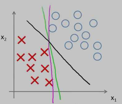
黑色的那条 decision boundary 的优点是:有着更大的 margin。这就是SVM分类器的特点:总是尽可能地找出一条最大 margin 的decision boundary,因此SVM有时也称为 Large Margin Classifier。
对于下图中的数据(有一个红色的叉很“奇特”),SVM又会怎样寻找 decision boundary呢?
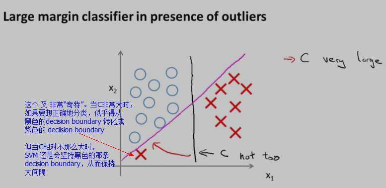
当SVM的代价函数中的C不是太大的情况下,SVM还是会坚持黑色那条decision boundary,而不是转化成紫色的那条 decision boundary。
当SVM的代价函数中的参数C很大时,它就很可能会选择紫色的那条 decision boundary了。但是,在实际应用上,C 不会是 很大很大的,因此,尽管样本中出现了“奇异点”样本,SVM还是会坚持黑色那条decision boundary,从而具有一定的“容错性”
③SVM为什么是大间距分类器?(Why Large Margin?)
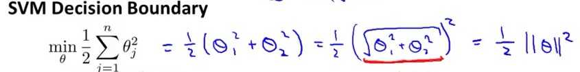
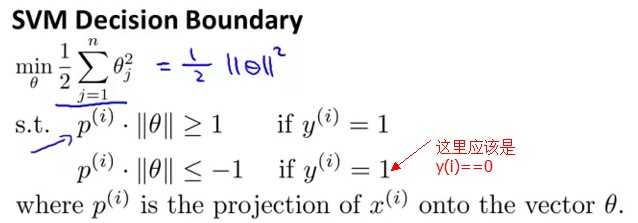
假设当C很大时,代价函数:min (1/2)·Σθ2j 可以表示成向量的乘法形式:min (1/2)θT·θ
因为:Σθj2 = (θ12 +θ22 +.... +θn2) = (θ1,θ2,....,θn)T? (θ1,θ2,....,θn) = ||θ||2
因此,我们把代价函数 转化成了:向量θ的范数,如下图 (n=2)
在最小化代价函数时,服从于下面条件:
θT·x(i)  >= 1    if  y==1
θT·x(i) <= -1    if y==0
向量乘法与向量投影之间的关系:假设有两个向量a,向量b;向量a、b之间的夹角为theta,由向量乘法公式:a*b=||a||*||b||*cos(theta)。其实,||b||*cos(theta)就是向量b在向量a上的投影。
根据向量的投影,θT·x(i) = p(i)?||θ||,其中p(i)是向量 x(i) 在 向量θ 方向上的投影。θT·x(i) = p(i)?||θ|| 的示意图如下:
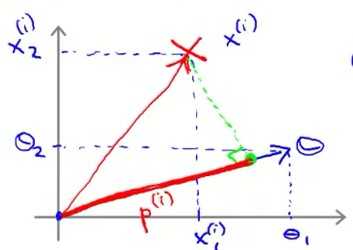
从而,将代价函数服从的条件转化成了“向量投影”表示,如下:
要想最小化代价函数(1/2)·Σθ2j ,就得让||θ||尽可能地小;但是又得满足条件:θT·x(i) >= 1 if y==1 and θT·x(i) <= -1 if y==0
根据:θT·x(i) = p(i)?||θ||。因此,要想θT·x(i) 尽可能地大于等于 1 ,就得让p(i) 尽可能地大,这样p(i)?||θ|| 才有更大的可能 大于等于1。
(不能让||θ||尽可能地大,因为||θ||大了,代价函数就大了,而我们的目标是最小化代价函数)
好,既然现在的目标是让p(i)尽可能地大,那p(i)代表的意义是什么呢?就是:margins(间距),这也是SVM被称为 大间距分类器 的原因。
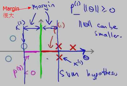
那 p(i) 为什么代表的是间距呢?看下图:
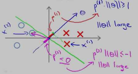
红色的叉叉 和 圆圈 表示的是训练的样本,我们用一条绿色的线(decision boundary)将叉叉 和 圆圈 分开。向量θ 的方向是与decision boundary 垂直的。
对于“红色的叉叉”这个样本x(1)而言,它的几何间距是 p(1);对于圆圈样本 x(2) 而言,它的几何间距是p(2)
从上图中可以看出,p(1) 和p(2) 的长度 都比较短,因此,要想让p(i)?||θ|| 大于等于1 或者 小于等于-1,只能让||θ||大一点了,而||θ||要是很大,代价函数就大了,而最小化SVM的代价函数的意义就是:找出一组参数(θ1,θ2......θn),使得代价函数尽可能地小。因此,SVM是不会选择 p(1) 长度 小的 decision boundary的。
再来看一个投影长度p(i) 比较长的例子:
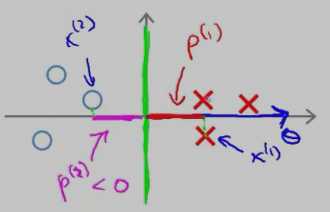
红色的叉叉 和 圆圈 表示的是训练的样本,我们用一条绿色的线(decision boundary)将叉叉 和 圆圈 分开,此时的decision boundary刚好是 y 轴(竖直线);红色的叉叉样本x(1) 在向量上的投影p(1 )刚好是x(1) 的 x 轴的坐标,它要比斜着的绿色decision boundary 上的投影 要长。
因此,SVM 会选择这条竖直的绿色 decision boundary 作为分类边界。它的 Margin 的示意图如下:
在上面的描述中,我们是先假设 SVM 的cost function 中的参数 C 很大,只留下了 θ(min (1/2)·Σθ2j )。然后根据 样本x(i) 在 θ向量上 的投影尽可能大 使得Margin很大,从而选择Margin大的 decision boundary,下面将从另一个角度来讨论为什么选择大的 margins(参考 cs229-notes3.pdf)
首先看下图中的一个线性可分的例子:
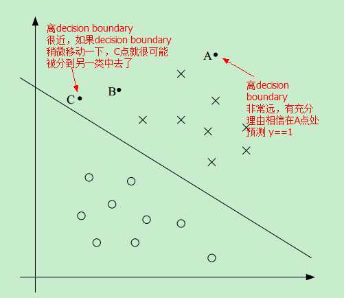
因此,如果我们能找到这样一条 decision boundary,让所有的点尽可能地离该decision boundary 远,这样我们就更有理由预测 y==1 或者 y==0
比如,相比于C点,我们更有理由相信 A点属于 positive 这一类,即更相信 预测 A点的 y==1 而不是预测C点的 y==1
简便起见,我们只考虑线性可分的二分类问题,y==1 或者 y==-1 来标记样本属于不同的分类。
we’ll use y ∈ {?1, 1} (instead of {0, 1}) to denote the class labels
待完成
④核函数(主要讨论高斯核函数)(待完成)
We’ll also see kernels, which give a way to apply SVMs efficiently in very high dimensional
(such as infinitedimensional) feature spaces
使用SVM实现垃圾邮件分类器
?输入数据(邮件)预处理并构造样本特征(input features)
假设一份样本邮件如下:

> Anyone knows how much it costs to host a web portal ?
>
Well, it depends on how many visitors you‘re expecting.
This can be anywhere from less than 10 bucks a month to a couple of $100.
You should checkout http://www.rackspace.com/ or perhaps Amazon EC2
if youre running something big..

To unsubscribe yourself from this mailing list, send an email to:
groupname-unsubscribe@egroups.com
这份样本邮件中有:URL、邮件地址、数字、金额(dollar)....这些特征都是与特定的Email相关的。对于不同的Email,也许也有URL、邮件地址.....但只是URL地址不一样,邮件地址不一样、出现的金额不一样.....因此,就需要“normalize”这些值,也就是说:我们关注的还是URL地址是什么,金额是多少,我们关注的是:是否出现了URL,是否出现了邮件地址....预处理策略如下:
比如,所有的URL 都用字符串“httpaddr”代替;所有的邮件地址都用字符串“emailaddr”代替;邮件中的所有的大写字母都转换成小写字母....
处理完之后,邮件变成了如下:
anyon know how much it cost to host a web portal well it depend on how mani
visitor you re expect thi can be anywher from less than number buck a month
to a coupl of dollarnumb you should checkout httpaddr or perhap amazon ecnumb
if your run someth big to unsubscrib yourself from thi mail list send an
email to emailaddr
在本例中,我们有一个词库,这个词库有1899个单词,因此 input features 是一个1899维的向量
如果处理之后的邮件中的单词出现在了词库中,input features 对应的位置为1,否则为0
processEmail.m用来进行上述预处理,其代码如下:

function word_indices = processEmail(email_contents)
%PROCESSEMAIL preprocesses a the body of an email and
%returns a list of word_indices
%   word_indices = PROCESSEMAIL(email_contents) preprocesses
%   the body of an email and returns a list of indices of the
%   words contained in the email.
%

% Load Vocabulary
vocabList = getVocabList();

% Init return value
word_indices = [];

% ========================== Preprocess Email ===========================

% Find the Headers ( \n\n and remove )
% Uncomment the following lines if you are working with raw emails with the
% full headers

% hdrstart = strfind(email_contents, ([char(10) char(10)]));
% email_contents = email_contents(hdrstart(1):end);

% Lower case
email_contents = lower(email_contents);

% Strip all HTML
% Looks for any expression that starts with < and ends with > and replace
% and does not have any < or > in the tag it with a space
email_contents = regexprep(email_contents, ‘<[^<>]+>‘, ‘ ‘);

% Handle Numbers
% Look for one or more characters between 0-9
email_contents = regexprep(email_contents, ‘[0-9]+‘, ‘number‘);

% Handle URLS
% Look for strings starting with http:// or https://
email_contents = regexprep(email_contents, ...
                           ‘(http|https)://[^\s]*‘, ‘httpaddr‘);

% Handle Email Addresses
% Look for strings with @ in the middle
email_contents = regexprep(email_contents, ‘[^\s]+@[^\s]+‘, ‘emailaddr‘);

% Handle $ sign
email_contents = regexprep(email_contents, ‘[$]+‘, ‘dollar‘);


% ========================== Tokenize Email ===========================

% Output the email to screen as well
fprintf(‘\n==== Processed Email ====\n\n‘);

% Process file
l = 0;

while ~isempty(email_contents)

    % Tokenize and also get rid of any punctuation
    [str, email_contents] = ...
       strtok(email_contents, ...
              [‘ @$/#.-:&*+=[]?!(){},‘‘">_<;%‘ char(10) char(13)]);

    % Remove any non alphanumeric characters
    str = regexprep(str, ‘[^a-zA-Z0-9]‘, ‘‘);

    % Stem the word
    % (the porterStemmer sometimes has issues, so we use a try catch block)
    try str = porterStemmer(strtrim(str));
    catch str = ‘‘; continue;
    end;

    % Skip the word if it is too short
    if length(str) < 1
       continue;
    end

    % Look up the word in the dictionary and add to word_indices if
    % found
    % ====================== YOUR CODE HERE ======================
    % Instructions: Fill in this function to add the index of str to
    %               word_indices if it is in the vocabulary. At this point
    %               of the code, you have a stemmed word from the email in
    %               the variable str. You should look up str in the
    %               vocabulary list (vocabList). If a match exists, you
    %               should add the index of the word to the word_indices
    %               vector. Concretely, if str = ‘action‘, then you should
    %               look up the vocabulary list to find where in vocabList
    %               ‘action‘ appears. For example, if vocabList{18} =
    %               ‘action‘, then, you should add 18 to the word_indices
    %               vector (e.g., word_indices = [word_indices ; 18]; ).
    %
    % Note: vocabList{idx} returns a the word with index idx in the
    %       vocabulary list.
    %
    % Note: You can use strcmp(str1, str2) to compare two strings (str1 and
    %       str2). It will return 1 only if the two strings are equivalent.
    %

    for i = 1:length(vocabList)
        if(strcmp(str, vocabList{i}) == 1)
            word_indices = [word_indices; i];
            break;
        end
    end
    % =============================================================


    % Print to screen, ensuring that the output lines are not too long
    if (l + length(str) + 1) > 78
        fprintf(‘\n‘);
        l = 0;
    end
    fprintf(‘%s ‘, str);
    l = l + length(str) + 1;

end

% Print footer
fprintf(‘\n\n=========================\n‘);

end
预处理的结果如下:
Length of feature vector: 1899
Number of non-zero entries: 45
表明:在上面的那封邮件中,有45个单词出现在词库中。
?训练SVM
spamTrain.mat 中包含了4000封邮件(即有垃圾邮件,也有非垃圾邮件),spamTest.mat中包含了1000个测试样本,相应的训练代码如下:
%% =========== Part 3: Train Linear SVM for Spam Classification ========
%  In this section, you will train a linear classifier to determine if an
%  email is Spam or Not-Spam.

% Load the Spam Email dataset
% You will have X, y in your environment
load(‘spamTrain.mat‘);

fprintf(‘\nTraining Linear SVM (Spam Classification)\n‘)
fprintf(‘(this may take 1 to 2 minutes) ...\n‘)

C = 0.1;
model = svmTrain(X, y, C, @linearKernel);

p = svmPredict(model, X);

fprintf(‘Training Accuracy: %f\n‘, mean(double(p == y)) * 100);
svmTrain 实现了SMO算法,svmTrain.m代码如下:
function [model] = svmTrain(X, Y, C, kernelFunction, ...
                            tol, max_passes)
%SVMTRAIN Trains an SVM classifier using a simplified version of the SMO
%algorithm.
%   [model] = SVMTRAIN(X, Y, C, kernelFunction, tol, max_passes) trains an
%   SVM classifier and returns trained model. X is the matrix of training
%   examples.  Each row is a training example, and the jth column holds the
%   jth feature.  Y is a column matrix containing 1 for positive examples
%   and 0 for negative examples.  C is the standard SVM regularization
%   parameter.  tol is a tolerance value used for determining equality of
%   floating point numbers. max_passes controls the number of iterations
%   over the dataset (without changes to alpha) before the algorithm quits.
%
% Note: This is a simplified version of the SMO algorithm for training
%       SVMs. In practice, if you want to train an SVM classifier, we
%       recommend using an optimized package such as:
%
%           LIBSVM   (http://www.csie.ntu.edu.tw/~cjlin/libsvm/)
%           SVMLight (http://svmlight.joachims.org/)
%
%

if ~exist(‘tol‘, ‘var‘) || isempty(tol)
    tol = 1e-3;
end

if ~exist(‘max_passes‘, ‘var‘) || isempty(max_passes)
    max_passes = 5;
end

% Data parameters
m = size(X, 1);
n = size(X, 2);

% Map 0 to -1
Y(Y==0) = -1;

% Variables
alphas = zeros(m, 1);
b = 0;
E = zeros(m, 1);
passes = 0;
eta = 0;
L = 0;
H = 0;

% Pre-compute the Kernel Matrix since our dataset is small
% (in practice, optimized SVM packages that handle large datasets
%  gracefully will _not_ do this)
%
% We have implemented optimized vectorized version of the Kernels here so
% that the svm training will run faster.
if strcmp(func2str(kernelFunction), ‘linearKernel‘)
    % Vectorized computation for the Linear Kernel
    % This is equivalent to computing the kernel on every pair of examples
    K = X*X‘;
elseif strfind(func2str(kernelFunction), ‘gaussianKernel‘)
    % Vectorized RBF Kernel
    % This is equivalent to computing the kernel on every pair of examples
    X2 = sum(X.^2, 2);
    K = bsxfun(@plus, X2, bsxfun(@plus, X2‘, - 2 * (X * X‘)));
    K = kernelFunction(1, 0) .^ K;
else
    % Pre-compute the Kernel Matrix
    % The following can be slow due to the lack of vectorization
    K = zeros(m);
    for i = 1:m
        for j = i:m
             K(i,j) = kernelFunction(X(i,:)‘, X(j,:)‘);
             K(j,i) = K(i,j); %the matrix is symmetric
        end
    end
end

% Train
fprintf(‘\nTraining ...‘);
dots = 12;
while passes < max_passes,

    num_changed_alphas = 0;
    for i = 1:m,

        % Calculate Ei = f(x(i)) - y(i) using (2).
        % E(i) = b + sum (X(i, :) * (repmat(alphas.*Y,1,n).*X)‘) - Y(i);
        E(i) = b + sum (alphas.*Y.*K(:,i)) - Y(i);

        if ((Y(i)*E(i) < -tol && alphas(i) < C) || (Y(i)*E(i) > tol && alphas(i) > 0)),

            % In practice, there are many heuristics one can use to select
            % the i and j. In this simplified code, we select them randomly.
            j = ceil(m * rand());
            while j == i,  % Make sure i \neq j
                j = ceil(m * rand());
            end

            % Calculate Ej = f(x(j)) - y(j) using (2).
            E(j) = b + sum (alphas.*Y.*K(:,j)) - Y(j);

            % Save old alphas
            alpha_i_old = alphas(i);
            alpha_j_old = alphas(j);

            % Compute L and H by (10) or (11).
            if (Y(i) == Y(j)),
                L = max(0, alphas(j) + alphas(i) - C);
                H = min(C, alphas(j) + alphas(i));
            else
                L = max(0, alphas(j) - alphas(i));
                H = min(C, C + alphas(j) - alphas(i));
            end

            if (L == H),
                % continue to next i.
                continue;
            end

            % Compute eta by (14).
            eta = 2 * K(i,j) - K(i,i) - K(j,j);
            if (eta >= 0),
                % continue to next i.
                continue;
            end

            % Compute and clip new value for alpha j using (12) and (15).
            alphas(j) = alphas(j) - (Y(j) * (E(i) - E(j))) / eta;

            % Clip
            alphas(j) = min (H, alphas(j));
            alphas(j) = max (L, alphas(j));

            % Check if change in alpha is significant
            if (abs(alphas(j) - alpha_j_old) < tol),
                % continue to next i.
                % replace anyway
                alphas(j) = alpha_j_old;
                continue;
            end

            % Determine value for alpha i using (16).
            alphas(i) = alphas(i) + Y(i)*Y(j)*(alpha_j_old - alphas(j));

            % Compute b1 and b2 using (17) and (18) respectively.
            b1 = b - E(i) ...
                 - Y(i) * (alphas(i) - alpha_i_old) *  K(i,j)‘ ...
                 - Y(j) * (alphas(j) - alpha_j_old) *  K(i,j)‘;
            b2 = b - E(j) ...
                 - Y(i) * (alphas(i) - alpha_i_old) *  K(i,j)‘ ...
                 - Y(j) * (alphas(j) - alpha_j_old) *  K(j,j)‘;

            % Compute b by (19).
            if (0 < alphas(i) && alphas(i) < C),
                b = b1;
            elseif (0 < alphas(j) && alphas(j) < C),
                b = b2;
            else
                b = (b1+b2)/2;
            end

            num_changed_alphas = num_changed_alphas + 1;

        end

    end

    if (num_changed_alphas == 0),
        passes = passes + 1;
    else
        passes = 0;
    end

    fprintf(‘.‘);
    dots = dots + 1;
    if dots > 78
        dots = 0;
        fprintf(‘\n‘);
    end
    if exist(‘OCTAVE_VERSION‘)
        fflush(stdout);
    end
end
fprintf(‘ Done! \n\n‘);

% Save the model
idx = alphas > 0;
model.X= X(idx,:);
model.y= Y(idx);
model.kernelFunction = kernelFunction;
model.b= b;
model.alphas= alphas(idx);
model.w = ((alphas.*Y)‘*X)‘;

end
训练的结果如下:
Training Accuracy: 99.850000

Evaluating the trained Linear SVM on a test set ...
Test Accuracy: 98.900000
?使用训练好的SVM分类进行邮件分类
%% =================== Part 6: Try Your Own Emails =====================
%  Now that you‘ve trained the spam classifier, you can use it on your own
%  emails! In the starter code, we have included spamSample1.txt,
%  spamSample2.txt, emailSample1.txt and emailSample2.txt as examples.
%  The following code reads in one of these emails and then uses your
%  learned SVM classifier to determine whether the email is Spam or
%  Not Spam

% Set the file to be read in (change this to spamSample2.txt,
% emailSample1.txt or emailSample2.txt to see different predictions on
% different emails types). Try your own emails as well!
filename = ‘emailSample1.txt‘;

% Read and predict
file_contents = readFile(filename);
word_indices  = processEmail(file_contents);
x             = emailFeatures(word_indices);
p = svmPredict(model, x);

fprintf(‘\nProcessed %s\n\nSpam Classification: %d\n‘, filename, p);
fprintf(‘(1 indicates spam, 0 indicates not spam)\n\n‘);
原文:http://www.cnblogs.com/hapjin/p/6140646.html