标签:figure oat lib color 相关 das center 1.4 图片
import pandas as pd
import numpy as np
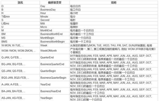
M:月
# TIMES的几种书写方式 #2016 Jul 1; 7/1/2016; 1/7/2016 ;2016-07-01; 2016/07/01
rng = pd.date_range(‘2016-07-01‘, periods = 10, freq = ‘3D‘)#不传freq则默认是D
rng
结果:

DatetimeIndex([‘2016-07-01‘, ‘2016-07-04‘, ‘2016-07-07‘, ‘2016-07-10‘,
               ‘2016-07-13‘, ‘2016-07-16‘, ‘2016-07-19‘, ‘2016-07-22‘,
               ‘2016-07-25‘, ‘2016-07-28‘],
              dtype=‘datetime64[ns]‘, freq=‘3D‘)
time=pd.Series(np.random.randn(20),
           index=pd.date_range(dt.datetime(2016,1,1),periods=20))
print(time)
#结果:
2016-01-01   -0.129379
2016-01-02    0.164480
2016-01-03   -0.639117
2016-01-04   -0.427224
2016-01-05    2.055133
2016-01-06    1.116075
2016-01-07    0.357426
2016-01-08    0.274249
2016-01-09    0.834405
2016-01-10   -0.005444
2016-01-11   -0.134409
2016-01-12    0.249318
2016-01-13   -0.297842
2016-01-14   -0.128514
2016-01-15    0.063690
2016-01-16   -2.246031
2016-01-17    0.359552
2016-01-18    0.383030
2016-01-19    0.402717
2016-01-20   -0.694068
Freq: D, dtype: float64
time.truncate(before=‘2016-1-10‘)#1月10之前的都被过滤掉了
结果:
2016-01-10   -0.005444
2016-01-11   -0.134409
2016-01-12    0.249318
2016-01-13   -0.297842
2016-01-14   -0.128514
2016-01-15    0.063690
2016-01-16   -2.246031
2016-01-17    0.359552
2016-01-18    0.383030
2016-01-19    0.402717
2016-01-20   -0.694068
Freq: D, dtype: float64
time.truncate(after=‘2016-1-10‘)#1月10之后的都被过滤掉了
#结果:
2016-01-01   -0.129379
2016-01-02    0.164480
2016-01-03   -0.639117
2016-01-04   -0.427224
2016-01-05    2.055133
2016-01-06    1.116075
2016-01-07    0.357426
2016-01-08    0.274249
2016-01-09    0.834405
2016-01-10   -0.005444
Freq: D, dtype: float64
print(time[‘2016-01-15‘])#0.063690487247
print(time[‘2016-01-15‘:‘2016-01-20‘])
结果:
2016-01-15    0.063690
2016-01-16   -2.246031
2016-01-17    0.359552
2016-01-18    0.383030
2016-01-19    0.402717
2016-01-20   -0.694068
Freq: D, dtype: float64


data=pd.date_range(‘2010-01-01‘,‘2011-01-01‘,freq=‘M‘)
print(data)
#结果:
DatetimeIndex([‘2010-01-31‘, ‘2010-02-28‘, ‘2010-03-31‘, ‘2010-04-30‘,
               ‘2010-05-31‘, ‘2010-06-30‘, ‘2010-07-31‘, ‘2010-08-31‘,
               ‘2010-09-30‘, ‘2010-10-31‘, ‘2010-11-30‘, ‘2010-12-31‘],
              dtype=‘datetime64[ns]‘, freq=‘M‘)
#时间戳
pd.Timestamp(‘2016-07-10‘)#Timestamp(‘2016-07-10 00:00:00‘)
# 可以指定更多细节
pd.Timestamp(‘2016-07-10 10‘)#Timestamp(‘2016-07-10 10:00:00‘)
pd.Timestamp(‘2016-07-10 10:15‘)#Timestamp(‘2016-07-10 10:15:00‘)

# How much detail can you add?
t = pd.Timestamp(‘2016-07-10 10:15‘)

# 时间区间
pd.Period(‘2016-01‘)#Period(‘2016-01‘, ‘M‘)
pd.Period(‘2016-01-01‘)#Period(‘2016-01-01‘, ‘D‘)

# TIME OFFSETS
pd.Timedelta(‘1 day‘)#Timedelta(‘1 days 00:00:00‘)
pd.Period(‘2016-01-01 10:10‘) + pd.Timedelta(‘1 day‘)#Period(‘2016-01-02 10:10‘, ‘T‘)
pd.Timestamp(‘2016-01-01 10:10‘) + pd.Timedelta(‘1 day‘)#Timestamp(‘2016-01-02 10:10:00‘)
pd.Timestamp(‘2016-01-01 10:10‘) + pd.Timedelta(‘15 ns‘)#Timestamp(‘2016-01-01 10:10:00.000000015‘)

p1 = pd.period_range(‘2016-01-01 10:10‘, freq = ‘25H‘, periods = 10)
p2 = pd.period_range(‘2016-01-01 10:10‘, freq = ‘1D1H‘, periods = 10)
p1
p2
结果:
PeriodIndex([‘2016-01-01 10:00‘, ‘2016-01-02 11:00‘, ‘2016-01-03 12:00‘,
             ‘2016-01-04 13:00‘, ‘2016-01-05 14:00‘, ‘2016-01-06 15:00‘,
             ‘2016-01-07 16:00‘, ‘2016-01-08 17:00‘, ‘2016-01-09 18:00‘,
             ‘2016-01-10 19:00‘],
            dtype=‘period[25H]‘, freq=‘25H‘)
PeriodIndex([‘2016-01-01 10:00‘, ‘2016-01-02 11:00‘, ‘2016-01-03 12:00‘,
             ‘2016-01-04 13:00‘, ‘2016-01-05 14:00‘, ‘2016-01-06 15:00‘,
             ‘2016-01-07 16:00‘, ‘2016-01-08 17:00‘, ‘2016-01-09 18:00‘,
             ‘2016-01-10 19:00‘],
            dtype=‘period[25H]‘, freq=‘25H‘)

# 指定索引
rng = pd.date_range(‘2016 Jul 1‘, periods = 10, freq = ‘D‘)
rng
pd.Series(range(len(rng)), index = rng)
结果:
2016-07-01    0
2016-07-02    1
2016-07-03    2
2016-07-04    3
2016-07-05    4
2016-07-06    5
2016-07-07    6
2016-07-08    7
2016-07-09    8
2016-07-10    9
Freq: D, dtype: int32

periods = [pd.Period(‘2016-01‘), pd.Period(‘2016-02‘), pd.Period(‘2016-03‘)]
ts = pd.Series(np.random.randn(len(periods)), index = periods)
ts
结果:
2016-01   -0.015837
2016-02   -0.923463
2016-03   -0.485212
Freq: M, dtype: float64

type(ts.index)#pandas.core.indexes.period.PeriodIndex

# 时间戳和时间周期可以转换
ts = pd.Series(range(10), pd.date_range(‘07-10-16 8:00‘, periods = 10, freq = ‘H‘))
ts
结果:
2016-07-10 08:00:00    0
2016-07-10 09:00:00    1
2016-07-10 10:00:00    2
2016-07-10 11:00:00    3
2016-07-10 12:00:00    4
2016-07-10 13:00:00    5
2016-07-10 14:00:00    6
2016-07-10 15:00:00    7
2016-07-10 16:00:00    8
2016-07-10 17:00:00    9
Freq: H, dtype: int32

ts_period = ts.to_period()
ts_period
结果:
2016-07-10 08:00    0
2016-07-10 09:00    1
2016-07-10 10:00    2
2016-07-10 11:00    3
2016-07-10 12:00    4
2016-07-10 13:00    5
2016-07-10 14:00    6
2016-07-10 15:00    7
2016-07-10 16:00    8
2016-07-10 17:00    9
Freq: H, dtype: int32

时间周期与时间戳的区别

ts_period[‘2016-07-10 08:30‘:‘2016-07-10 11:45‘] #时间周期包含08:00
结果:
2016-07-10 08:00    0
2016-07-10 09:00    1
2016-07-10 10:00    2
2016-07-10 11:00    3
Freq: H, dtype: int32

ts[‘2016-07-10 08:30‘:‘2016-07-10 11:45‘] #时间戳不包含08:30
#结果:
2016-07-10 09:00:00    1
2016-07-10 10:00:00    2
2016-07-10 11:00:00    3
Freq: H, dtype: int32
import pandas as pd
import numpy as np
rng = pd.date_range(‘1/1/2011‘, periods=90, freq=‘D‘)#数据按天
ts = pd.Series(np.random.randn(len(rng)), index=rng)
ts.head()
结果:
2011-01-01   -1.025562
2011-01-02    0.410895
2011-01-03    0.660311
2011-01-04    0.710293
2011-01-05    0.444985
Freq: D, dtype: float64

ts.resample(‘M‘).sum()#数据降采样,降为月,指标是求和,也可以平均,自己指定
结果:
2011-01-31    2.510102
2011-02-28    0.583209
2011-03-31    2.749411
Freq: M, dtype: float64

ts.resample(‘3D‘).sum()#数据降采样,降为3天
结果:
2011-01-01    0.045643
2011-01-04   -2.255206
2011-01-07    0.571142
2011-01-10    0.835032
2011-01-13   -0.396766
2011-01-16   -1.156253
2011-01-19   -1.286884
2011-01-22    2.883952
2011-01-25    1.566908
2011-01-28    1.435563
2011-01-31    0.311565
2011-02-03   -2.541235
2011-02-06    0.317075
2011-02-09    1.598877
2011-02-12   -1.950509
2011-02-15    2.928312
2011-02-18   -0.733715
2011-02-21    1.674817
2011-02-24   -2.078872
2011-02-27    2.172320
2011-03-02   -2.022104
2011-03-05   -0.070356
2011-03-08    1.276671
2011-03-11   -2.835132
2011-03-14   -1.384113
2011-03-17    1.517565
2011-03-20   -0.550406
2011-03-23    0.773430
2011-03-26    2.244319
2011-03-29    2.951082
Freq: 3D, dtype: float64

day3Ts = ts.resample(‘3D‘).mean()
day3Ts
结果:
2011-01-01    0.015214
2011-01-04   -0.751735
2011-01-07    0.190381
2011-01-10    0.278344
2011-01-13   -0.132255
2011-01-16   -0.385418
2011-01-19   -0.428961
2011-01-22    0.961317
2011-01-25    0.522303
2011-01-28    0.478521
2011-01-31    0.103855
2011-02-03   -0.847078
2011-02-06    0.105692
2011-02-09    0.532959
2011-02-12   -0.650170
2011-02-15    0.976104
2011-02-18   -0.244572
2011-02-21    0.558272
2011-02-24   -0.692957
2011-02-27    0.724107
2011-03-02   -0.674035
2011-03-05   -0.023452
2011-03-08    0.425557
2011-03-11   -0.945044
2011-03-14   -0.461371
2011-03-17    0.505855
2011-03-20   -0.183469
2011-03-23    0.257810
2011-03-26    0.748106
2011-03-29    0.983694
Freq: 3D, dtype: float64

print(day3Ts.resample(‘D‘).asfreq())#升采样,要进行插值
结果:
2011-01-01    0.015214
2011-01-02         NaN
2011-01-03         NaN
2011-01-04   -0.751735
2011-01-05         NaN
2011-01-06         NaN
2011-01-07    0.190381
2011-01-08         NaN
2011-01-09         NaN
2011-01-10    0.278344
2011-01-11         NaN
2011-01-12         NaN
2011-01-13   -0.132255
2011-01-14         NaN
2011-01-15         NaN
2011-01-16   -0.385418
2011-01-17         NaN
2011-01-18         NaN
2011-01-19   -0.428961
2011-01-20         NaN
2011-01-21         NaN
2011-01-22    0.961317
2011-01-23         NaN
2011-01-24         NaN
2011-01-25    0.522303
2011-01-26         NaN
2011-01-27         NaN
2011-01-28    0.478521
2011-01-29         NaN
2011-01-30         NaN
                ...
2011-02-28         NaN
2011-03-01         NaN
2011-03-02   -0.674035
2011-03-03         NaN
2011-03-04         NaN
2011-03-05   -0.023452
2011-03-06         NaN
2011-03-07         NaN
2011-03-08    0.425557
2011-03-09         NaN
2011-03-10         NaN
2011-03-11   -0.945044
2011-03-12         NaN
2011-03-13         NaN
2011-03-14   -0.461371
2011-03-15         NaN
2011-03-16         NaN
2011-03-17    0.505855
2011-03-18         NaN
2011-03-19         NaN
2011-03-20   -0.183469
2011-03-21         NaN
2011-03-22         NaN
2011-03-23    0.257810
2011-03-24         NaN
2011-03-25         NaN
2011-03-26    0.748106
2011-03-27         NaN
2011-03-28         NaN
2011-03-29    0.983694
Freq: D, Length: 88, dtype: float64
day3Ts.resample(‘D‘).ffill(1)
结果:
2011-01-01    0.015214
2011-01-02    0.015214
2011-01-03         NaN
2011-01-04   -0.751735
2011-01-05   -0.751735
2011-01-06         NaN
2011-01-07    0.190381
2011-01-08    0.190381
2011-01-09         NaN
2011-01-10    0.278344
2011-01-11    0.278344
2011-01-12         NaN
2011-01-13   -0.132255
2011-01-14   -0.132255
2011-01-15         NaN
2011-01-16   -0.385418
2011-01-17   -0.385418
2011-01-18         NaN
2011-01-19   -0.428961
2011-01-20   -0.428961
2011-01-21         NaN
2011-01-22    0.961317
2011-01-23    0.961317
2011-01-24         NaN
2011-01-25    0.522303
2011-01-26    0.522303
2011-01-27         NaN
2011-01-28    0.478521
2011-01-29    0.478521
2011-01-30         NaN
                ...
2011-02-28    0.724107
2011-03-01         NaN
2011-03-02   -0.674035
2011-03-03   -0.674035
2011-03-04         NaN
2011-03-05   -0.023452
2011-03-06   -0.023452
2011-03-07         NaN
2011-03-08    0.425557
2011-03-09    0.425557
2011-03-10         NaN
2011-03-11   -0.945044
2011-03-12   -0.945044
2011-03-13         NaN
2011-03-14   -0.461371
2011-03-15   -0.461371
2011-03-16         NaN
2011-03-17    0.505855
2011-03-18    0.505855
2011-03-19         NaN
2011-03-20   -0.183469
2011-03-21   -0.183469
2011-03-22         NaN
2011-03-23    0.257810
2011-03-24    0.257810
2011-03-25         NaN
2011-03-26    0.748106
2011-03-27    0.748106
2011-03-28         NaN
2011-03-29    0.983694
Freq: D, Length: 88, dtype: float64

day3Ts.resample(‘D‘).bfill(1)
结果:
2011-01-01    0.015214
2011-01-02         NaN
2011-01-03   -0.751735
2011-01-04   -0.751735
2011-01-05         NaN
2011-01-06    0.190381
2011-01-07    0.190381
2011-01-08         NaN
2011-01-09    0.278344
2011-01-10    0.278344
2011-01-11         NaN
2011-01-12   -0.132255
2011-01-13   -0.132255
2011-01-14         NaN
2011-01-15   -0.385418
2011-01-16   -0.385418
2011-01-17         NaN
2011-01-18   -0.428961
2011-01-19   -0.428961
2011-01-20         NaN
2011-01-21    0.961317
2011-01-22    0.961317
2011-01-23         NaN
2011-01-24    0.522303
2011-01-25    0.522303
2011-01-26         NaN
2011-01-27    0.478521
2011-01-28    0.478521
2011-01-29         NaN
2011-01-30    0.103855
                ...
2011-02-28         NaN
2011-03-01   -0.674035
2011-03-02   -0.674035
2011-03-03         NaN
2011-03-04   -0.023452
2011-03-05   -0.023452
2011-03-06         NaN
2011-03-07    0.425557
2011-03-08    0.425557
2011-03-09         NaN
2011-03-10   -0.945044
2011-03-11   -0.945044
2011-03-12         NaN
2011-03-13   -0.461371
2011-03-14   -0.461371
2011-03-15         NaN
2011-03-16    0.505855
2011-03-17    0.505855
2011-03-18         NaN
2011-03-19   -0.183469
2011-03-20   -0.183469
2011-03-21         NaN
2011-03-22    0.257810
2011-03-23    0.257810
2011-03-24         NaN
2011-03-25    0.748106
2011-03-26    0.748106
2011-03-27         NaN
2011-03-28    0.983694
2011-03-29    0.983694
Freq: D, Length: 88, dtype: float64

day3Ts.resample(‘D‘).interpolate(‘linear‘)#线性拟合填充
结果:
2011-01-01    0.015214
2011-01-02   -0.240435
2011-01-03   -0.496085
2011-01-04   -0.751735
2011-01-05   -0.437697
2011-01-06   -0.123658
2011-01-07    0.190381
2011-01-08    0.219702
2011-01-09    0.249023
2011-01-10    0.278344
2011-01-11    0.141478
2011-01-12    0.004611
2011-01-13   -0.132255
2011-01-14   -0.216643
2011-01-15   -0.301030
2011-01-16   -0.385418
2011-01-17   -0.399932
2011-01-18   -0.414447
2011-01-19   -0.428961
2011-01-20    0.034465
2011-01-21    0.497891
2011-01-22    0.961317
2011-01-23    0.814979
2011-01-24    0.668641
2011-01-25    0.522303
2011-01-26    0.507709
2011-01-27    0.493115
2011-01-28    0.478521
2011-01-29    0.353632
2011-01-30    0.228744
                ...
2011-02-28    0.258060
2011-03-01   -0.207988
2011-03-02   -0.674035
2011-03-03   -0.457174
2011-03-04   -0.240313
2011-03-05   -0.023452
2011-03-06    0.126218
2011-03-07    0.275887
2011-03-08    0.425557
2011-03-09   -0.031310
2011-03-10   -0.488177
2011-03-11   -0.945044
2011-03-12   -0.783820
2011-03-13   -0.622595
2011-03-14   -0.461371
2011-03-15   -0.138962
2011-03-16    0.183446
2011-03-17    0.505855
2011-03-18    0.276080
2011-03-19    0.046306
2011-03-20   -0.183469
2011-03-21   -0.036376
2011-03-22    0.110717
2011-03-23    0.257810
2011-03-24    0.421242
2011-03-25    0.584674
2011-03-26    0.748106
2011-03-27    0.826636
2011-03-28    0.905165
2011-03-29    0.983694
Freq: D, Length: 88, dtype: float64
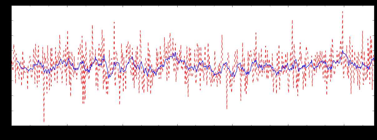
滑动窗口就是能够根据指定的单位长度来框住时间序列,从而计算框内的统计指标。相当于一个长度指定的滑块在刻度尺上面滑动,每滑动一个单位即可反馈滑块内的数据。
滑动窗口可以使数据更加平稳,浮动范围会比较小,具有代表性,单独拿出一个数据可能或多或少会离群,有差异或者错误,使用滑动窗口会更规范一些。
%matplotlib inline
import matplotlib.pylab
import numpy as np
import pandas as pd
df = pd.Series(np.random.randn(600), index = pd.date_range(‘7/1/2016‘, freq = ‘D‘, periods = 600))
df.head()
结果:
2016-07-01   -0.192140
2016-07-02    0.357953
2016-07-03   -0.201847
2016-07-04   -0.372230
2016-07-05    1.414753
Freq: D, dtype: float64

r = df.rolling(window = 10)
r#Rolling [window=10,center=False,axis=0]

#r.max, r.median, r.std, r.skew倾斜度, r.sum, r.var
print(r.mean())
结果:
2016-07-01         NaN
2016-07-02         NaN
2016-07-03         NaN
2016-07-04         NaN
2016-07-05         NaN
2016-07-06         NaN
2016-07-07         NaN
2016-07-08         NaN
2016-07-09         NaN
2016-07-10    0.300133
2016-07-11    0.284780
2016-07-12    0.252831
2016-07-13    0.220699
2016-07-14    0.167137
2016-07-15    0.018593
2016-07-16   -0.061414
2016-07-17   -0.134593
2016-07-18   -0.153333
2016-07-19   -0.218928
2016-07-20   -0.169426
2016-07-21   -0.219747
2016-07-22   -0.181266
2016-07-23   -0.173674
2016-07-24   -0.130629
2016-07-25   -0.166730
2016-07-26   -0.233044
2016-07-27   -0.256642
2016-07-28   -0.280738
2016-07-29   -0.289893
2016-07-30   -0.379625
                ...
2018-01-22   -0.211467
2018-01-23    0.034996
2018-01-24   -0.105910
2018-01-25   -0.145774
2018-01-26   -0.089320
2018-01-27   -0.164370
2018-01-28   -0.110892
2018-01-29   -0.205786
2018-01-30   -0.101162
2018-01-31   -0.034760
2018-02-01    0.229333
2018-02-02    0.043741
2018-02-03    0.052837
2018-02-04    0.057746
2018-02-05   -0.071401
2018-02-06   -0.011153
2018-02-07   -0.045737
2018-02-08   -0.021983
2018-02-09   -0.196715
2018-02-10   -0.063721
2018-02-11   -0.289452
2018-02-12   -0.050946
2018-02-13   -0.047014
2018-02-14    0.048754
2018-02-15    0.143949
2018-02-16    0.424823
2018-02-17    0.361878
2018-02-18    0.363235
2018-02-19    0.517436
2018-02-20    0.368020
Freq: D, Length: 600, dtype: float64

import matplotlib.pyplot as plt
%matplotlib inline

plt.figure(figsize=(15, 5))

df.plot(style=‘r--‘)
df.rolling(window=10).mean().plot(style=‘b‘)#<matplotlib.axes._subplots.AxesSubplot at 0x249627fb6d8>
结果:

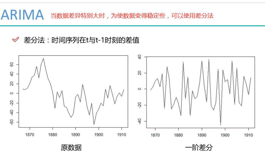
二阶差分是指在一阶差分基础上再做一阶差分。


标签:figure oat lib color 相关 das center 1.4 图片
原文地址:https://www.cnblogs.com/tianqizhi/p/9277376.html
