目录
VGGNet网络结构
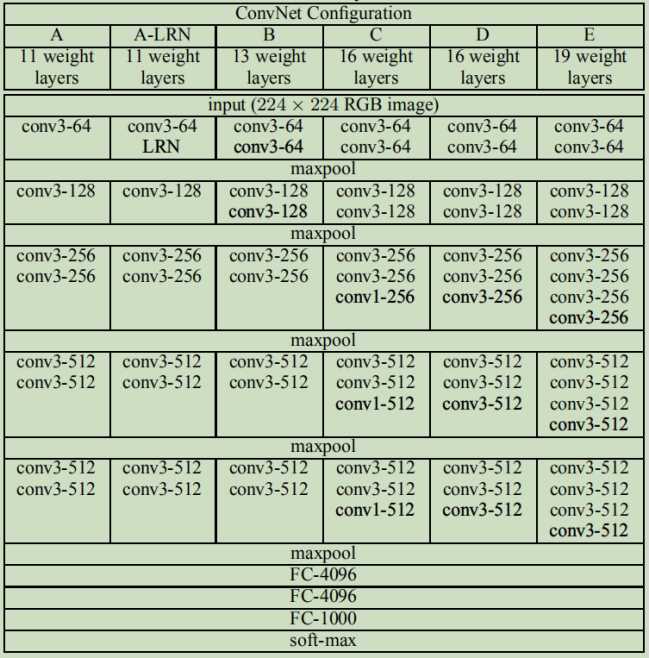
论文中还讨论了其他结构
参考资料
2014年,牛津大学计算机视觉组(Visual Geometry Group)和Google DeepMind公司的研究员一起研发出了新的深度卷积神经网络:VGGNet,并取得了ILSVRC2014比赛分类项目的第二名(第一名是GoogLeNet,也是同年提出的)和定位项目的第一名。
VGGNet探索了卷积神经网络的深度与其性能之间的关系,成功地构筑了16~19层深的卷积神经网络,证明了增加网络的深度能够在一定程度上影响网络最终的性能,使错误率大幅下降,同时拓展性又很强,迁移到其它图片数据上的泛化性也非常好。到目前为止,VGG仍然被用来提取图像特征。
VGGNet可以看成是加深版本的AlexNet,都是由卷积层、全连接层两大部分构成。
|
VGGNet网络结构 |
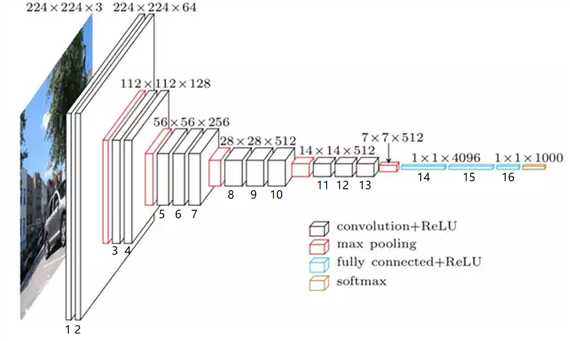
VGGNet比AlexNet的网络层数多,不再使用尺寸较大的卷积核,如11*11、7*7、5*5,而是只采用了尺寸为3*3的卷积核,VGG-16的卷积神经网络结构如下:
对应代码为:


import tensorflow as tf
import numpy as np

# 输入
x = tf.placeholder(tf.float32, [None, 224, 224, 3])
# 第1层:与64个3*3*3的核,步长=1,SAME卷积
w1 = tf.Variable(tf.random_normal([3, 3, 3, 64]), dtype=tf.float32, name=‘w1‘)
conv1 = tf.nn.relu(tf.nn.conv2d(x, w1, [1, 1, 1, 1], ‘SAME‘))
# 结果为224*224*64

# 第2层:与64个3*3*64的核,步长=1,SAME卷积
w2 = tf.Variable(tf.random_normal([3, 3, 64, 64]), dtype=tf.float32, name=‘w2‘)
conv2 = tf.nn.relu(tf.nn.conv2d(conv1, w2, [1, 1, 1, 1], ‘SAME‘))
# 结果为224*224*64

# 池化1
pool1 = tf.nn.max_pool(conv2, [1, 2, 2, 1], [1, 2, 2, 1], ‘VALID‘)
# 结果为112*112*64

# 第3层:与128个3*3*64的核,步长=1,SAME卷积
w3 = tf.Variable(tf.random_normal([3, 3, 64, 128]), dtype=tf.float32, name=‘w3‘)
conv3 = tf.nn.relu(tf.nn.conv2d(pool1, w3, [1, 1, 1, 1], ‘SAME‘))
# 结果为112*112*128

# 第4层:与128个3*3*128的核,步长=1,SAME卷积
w4 = tf.Variable(tf.random_normal([3, 3, 128, 128]), dtype=tf.float32, name=‘w4‘)
conv4 = tf.nn.relu(tf.nn.conv2d(conv3, w4, [1, 1, 1, 1], ‘SAME‘))
# 结果为112*112*128

# 池化2
pool2 = tf.nn.max_pool(conv4, [1, 2, 2, 1], [1, 2, 2, 1], ‘VALID‘)
# 结果为56*56*128

# 第5层:与256个3*3*128的核,步长=1,SAME卷积
w5 = tf.Variable(tf.random_normal([3, 3, 128, 256]), dtype=tf.float32, name=‘w5‘)
conv5 = tf.nn.relu(tf.nn.conv2d(pool2, w5, [1, 1, 1, 1], ‘SAME‘))
# 结果为56*56*256

# 第6层:与256个3*3*256的核,步长=1,SAME卷积
w6 = tf.Variable(tf.random_normal([3, 3, 256, 256]), dtype=tf.float32, name=‘w6‘)
conv6 = tf.nn.relu(tf.nn.conv2d(conv5, w6, [1, 1, 1, 1], ‘SAME‘))
# 结果为56*56*256

# 第7层:与256个3*3*256的核,步长=1,SAME卷积
w7 = tf.Variable(tf.random_normal([3, 3, 256, 256]), dtype=tf.float32, name=‘w7‘)
conv7 = tf.nn.relu(tf.nn.conv2d(conv6, w7, [1, 1, 1, 1], ‘SAME‘))
# 结果为56*56*256

# 池化3
pool3 = tf.nn.max_pool(conv7, [1, 2, 2, 1], [1, 2, 2, 1], ‘VALID‘)
# 结果为28*28*256

# 第8层:与512个3*3*256的核,步长=1,SAME卷积
w8 = tf.Variable(tf.random_normal([3, 3, 256, 512]), dtype=tf.float32, name=‘w8‘)
conv8 = tf.nn.relu(tf.nn.conv2d(pool3, w8, [1, 1, 1, 1], ‘SAME‘))
# 结果为28*28*512

# 第9层:与512个3*3*512的核,步长=1,SAME卷积
w9 = tf.Variable(tf.random_normal([3, 3, 512, 512]), dtype=tf.float32, name=‘w9‘)
conv9 = tf.nn.relu(tf.nn.conv2d(conv8, w9, [1, 1, 1, 1], ‘SAME‘))
# 结果为28*28*512

# 第10层:与512个3*3*512的核,步长=1,SAME卷积
w10 = tf.Variable(tf.random_normal([3, 3, 512, 512]), dtype=tf.float32, name=‘w10‘)
conv10 = tf.nn.relu(tf.nn.conv2d(conv9, w10, [1, 1, 1, 1], ‘SAME‘))
# 结果为28*28*512

# 池化4
pool4 = tf.nn.max_pool(conv10, [1, 2, 2, 1], [1, 2, 2, 1], ‘VALID‘)
# 结果为14*14*512

# 第11层:与512个3*3*256的核,步长=1,SAME卷积
w11 = tf.Variable(tf.random_normal([3, 3, 512, 512]), dtype=tf.float32, name=‘w11‘)
conv11 = tf.nn.relu(tf.nn.conv2d(pool4, w11, [1, 1, 1, 1], ‘SAME‘))
# 结果为14*14*512

# 第12层:与512个3*3*512的核,步长=1,SAME卷积
w12 = tf.Variable(tf.random_normal([3, 3, 512, 512]), dtype=tf.float32, name=‘w12‘)
conv12 = tf.nn.relu(tf.nn.conv2d(conv11, w12, [1, 1, 1, 1], ‘SAME‘))
# 结果为14*14*512

# 第13层:与512个3*3*512的核,步长=1,SAME卷积
w13 = tf.Variable(tf.random_normal([3, 3, 512, 512]), dtype=tf.float32, name=‘w13‘)
conv13 = tf.nn.relu(tf.nn.conv2d(conv12, w13, [1, 1, 1, 1], ‘SAME‘))
# 结果为14*14*512

# 池化5
pool5 = tf.nn.max_pool(conv13, [1, 2, 2, 1], [1, 2, 2, 1], ‘VALID‘)
# 结果为7*7*512

# 拉伸为25088
pool_l5_shape = pool5.get_shape()
num = pool_l5_shape[1].value * pool_l5_shape[2].value * pool_l5_shape[3].value
flatten = tf.reshape(pool5, [-1, num])
# 结果为25088*1

# 第14层:与4096个神经元全连接
fcW1 = tf.Variable(tf.random_normal([num, 4096]), dtype=tf.float32, name=‘fcW1‘)
fc1 = tf.nn.relu(tf.matmul(flatten, fcW1))

# 第15层:与4096个神经元全连接
fcW2 = tf.Variable(tf.random_normal([4096, 4096]), dtype=tf.float32, name=‘fcW2‘)
fc2 = tf.nn.relu(tf.matmul(fc1, fcW2))

# 第16层:与1000个神经元全连接+softmax输出
fcW3 = tf.Variable(tf.random_normal([4096, 1000]), dtype=tf.float32, name=‘fcW3‘)
out = tf.matmul(fc2, fcW3)
out=tf.nn.softmax(out)

session = tf.Session()
session.run(tf.global_variables_initializer())
result = session.run(out, feed_dict={x: np.ones([1, 224, 224, 3], np.float32)})
# "打印最后的输出尺寸"
print(np.shape(result))
|
论文中还讨论了其他结构 |
|
参考资料 |
吴恩达深度学习
VGGNet-Very Deep Convolutional Networks for Large-Scale Image Recognition
《图解深度学习与神经网络:从张量到TensorFlow实现》_张平
《深-度-学-习-核-心-技-术-与-实-践》
大话CNN经典模型:VGGNet
https://my.oschina.net/u/876354/blog/1634322