标签:经典 fonts wrap 朋友 ipy 有趣 隐藏 style pad

Seaborn和Matplotlib是Python最强大的两个可视化库。Seaborn其默认主题让人惊讶,而Matplotlib可以通过其多个分类为用户打造专属功能。

Python提供了各种用于绘制数据的包。本教程将使用以下两种包来演示Python的绘图功能:
· Matplotlib
· Seaborn

importmatplotlib.pyplot as plt
%matplotlib inline
import numpy as np
在上面的代码块中,将Pyplot模块调整为plt格式并导入Matplotliib库。这样做可以简化执行命令的过程,具体内容会在本篇教程中看到。PyPlot包含创建和编辑绘图所需的一系列命令。操作时同时运行%matplotlibinline,那么绘图下方就能自动显示代码块,否则用户每次绘图时都需要输入plt.show()来创建新图。此功能是Jupyter Notebook / IPython独有的。Matplotlib拥有定制的代码块结构,这使得它比其他绘图库更先进。接下来看看如何使用matploblib生成散点图。
提示:当使用matplotlib时,文本输出无法带来视觉上的吸引力。为了解决这个问题,我们在执行代码块生成图片时会在每一行代码末端添加分号“;”。
我们使用的数据库是UCI机器学习库中的共享单车数据集。
散点图是各种示意图中影响力最广、信息量最大、功能最多的一类图。它可以直接向用户传递信息,无需太多额外工作(如下图所示)。
· plt.scatter()将输入的散点图上的数据作为初始参数,其中temp指x轴,cnt指y轴。
· c指的是不同数据点的颜色。输入一个字符串“季节”,它也表示数据帧中的一列,不同颜色对应不同季节。该方法用可视化方法对数据分组,十分简单便捷。
plt.scatter(‘temp‘,‘cnt‘, data=day, c=‘season‘)
plt.xlabel(‘NormalizedTemperature‘, fontsize=‘large‘)
plt.ylabel(‘Countof Total Bike Rentals‘, fontsize=‘large‘);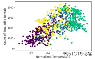
图上信息显示:
· 某些时间点的自行车租赁量超过8000辆。
· 标准温度超过0.8。
· 自行车租赁量与温度或季节无关。
· 自行车租赁量与标准温度之间含有正线性关系。
这个图的确含有大量信息,然而图表并不能产生图例,因此我们很难对各组季节数据进行破译。这是因为用散点图绘图时,Matplotlib无法根据绘图制作图例。下一节中,我们将会看到该图如何隐藏信息,甚至误导读者。
看看经过彻底编辑后的绘图。该图旨在根据不同组别绘制图例,并进行破译。
plt.rcParams[‘figure.figsize‘]= [15, 10]

fontdict={‘fontsize‘:18,
          ‘weight‘ : ‘bold‘,
         ‘horizontalalignment‘: ‘center‘}

fontdictx={‘fontsize‘:18,
          ‘weight‘ : ‘bold‘,
          ‘horizontalalignment‘: ‘center‘}

fontdicty={‘fontsize‘:16,
          ‘weight‘ : ‘bold‘,
          ‘verticalalignment‘: ‘baseline‘,
          ‘horizontalalignment‘: ‘center‘}

spring =plt.scatter(‘temp‘, ‘cnt‘, data=day[day[‘season‘]==1], marker=‘o‘,color=‘green‘)
summer =plt.scatter(‘temp‘, ‘cnt‘, data=day[day[‘season‘]==2], marker=‘o‘, color=‘orange‘)
autumn =plt.scatter(‘temp‘, ‘cnt‘, data=day[day[‘season‘]==3], marker=‘o‘,color=‘brown‘)
winter =plt.scatter(‘temp‘, ‘cnt‘, data=day[day[‘season‘]==4], marker=‘o‘,color=‘blue‘)
plt.legend(handles=(spring,summer,autumn,winter),
           labels=(‘Spring‘, ‘Summer‘,‘Fall/Autumn‘, ‘Winter‘),
           title="Season",title_fontsize=16,
           scatterpoints=1,
           bbox_to_anchor=(1, 0.7), loc=2,borderaxespad=1.,
           ncol=1,
           fontsize=14)
plt.title(‘BikeRentals at Different Temperatures\nBy Season‘, fontdict=fontdict,color="black")
plt.xlabel("Normalizedtemperature", fontdict=fontdictx)
plt.ylabel("Countof Total Rental Bikes", fontdict=fontdicty);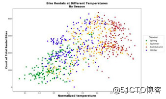
· plt.rcParams[‘figure.figsize‘]= [15, 10]限定了整张图的大小,这个代码对应的是一个长15厘米*宽10厘米的图。
· Fontdict是一个包含许多参数的字典,可以用于标记不同的轴,其中标题为fontdict,x轴为fontdictx,y轴为fontdicty。
· 如今有四个plt.scatter()函数,对应四个不同的季节,这一点在数据参数中再次出现,而这些数据参数已被子集化以对应不同单一季节。“o”表示不同的标记和颜色参数,这可以直观地显示数据点的位置以及其颜色。
· 在plt.legend()中输入参数形成图例。前两个参数是句柄:图例和标签会展示真正的散点图;而于各个图对应的名字也会在图例中出现。图上大小不一的标记代表散点,它们最终组合为一个散点图。bbox_to_anchor=(1, 0.7), loc=2, borderaxespad=1。这三个参数串联使用,来对照图例位置。点击这句话开头的链接,可以发现这些参数的本质。
现在可以通过区分不同季节来发现更多隐藏信息。但即使已经添加了额外的图层,散点图依然可以隐藏信息并带来误解。
该散点图:
· 数据中有重复部分。
· 分布混乱。
· 未显示自行车租赁在不同季节之间的明显差别。
· 隐藏信息,如:春夏气温上升时自行车出租量会增加。
· 表示自行车租赁量与气温呈正比关系。
· 并未清楚显示最低温出现在哪一季节。
创建子图可能是业界最具吸引力也是最专业的图表技术之一。当单一的图信息过多时,人们难以评估,子图就变得十分重要。
分面就是在同一个轴上绘制多个不同的图。分面是数据可视化中功能最多的技术之一。分面可以从多个角度展示信息,也可以揭露隐藏内容。
· 如前所述,plt.figure()将用于创建新的绘图画布。最终会保存为图画格式。
· 重复运行fig.add_subplot()代码4次,分别对应四个季节的子图。其参数则对应nrows,ncols和index。比方说axl对应图表上第一个绘图(索引在左上角从1开始,向右递增)。
· 余下的函数调用可以自我解释或被覆盖。
fig = plt.figure()

plt.rcParams[‘figure.figsize‘]= [15,10]
plt.rcParams["font.weight"]= "bold"

fontdict={‘fontsize‘:25,
          ‘weight‘ : ‘bold‘}

fontdicty={‘fontsize‘:18,
          ‘weight‘ : ‘bold‘,
          ‘verticalalignment‘: ‘baseline‘,
          ‘horizontalalignment‘: ‘center‘}

fontdictx={‘fontsize‘:18,
          ‘weight‘ : ‘bold‘,
          ‘horizontalalignment‘: ‘center‘}

plt.subplots_adjust(wspace=0.2,hspace=0.2)

fig.suptitle(‘BikeRentals at Different Temperatures\nBy Season‘,fontsize=25,fontweight="bold", color="black",
             position=(0.5,1.01))

ax1 =fig.add_subplot(221)
ax1.scatter(‘temp‘,‘cnt‘, data=day[day[‘season‘]==1], c="green")
ax1.set_title(‘Spring‘,fontdict=fontdict, color="green")
ax1.set_ylabel("Countof Total Rental Bikes", fontdict=fontdicty, position=(0,-0.1))

ax2 =fig.add_subplot(222)
ax2.scatter(‘temp‘,‘cnt‘, data=day[day[‘season‘]==2], c="orange")
ax2.set_title(‘Summer‘,fontdict=fontdict, color="orange")

ax3 =fig.add_subplot(223)
ax3.scatter(‘temp‘,‘cnt‘, data=day[day[‘season‘]==3], c="brown")
ax3.set_title(‘Fallor Autumn‘, fontdict=fontdict, color="brown")

ax4 =fig.add_subplot(224)
ax4.scatter(‘temp‘,‘cnt‘, data=day[day[‘season‘]==4], c="blue")
ax4.set_title("Winter",fontdict=fontdict, color="blue")
ax4.set_xlabel("Normalizedtemperature", fontdict=fontdictx, position=(-0.1,0));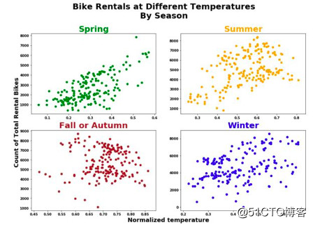
现在分别分析各组,效果也会更加显著。首先要注意到在不同季节里,自行车租赁量与气温的关系存在差异:
· 它们在春天呈现正线性关系。
· 它们在冬天和夏天呈二次非线性关系。
· 在秋天它们的正线性关系十分不明显。
但是,这些图依然有可能误导读者,原因也并不明显。四张图中,所有的轴都不一样。如果人们没有留意到这一点,那么他们很有可能会误解这些图。请参阅下文,了解如何解决该问题。
fig = plt.figure()

plt.rcParams[‘figure.figsize‘]= [12,12]
plt.rcParams["font.weight"]= "bold"

plt.subplots_adjust(hspace=0.60)

fontdicty={‘fontsize‘:20,
          ‘weight‘ : ‘bold‘,
          ‘verticalalignment‘: ‘baseline‘,
          ‘horizontalalignment‘: ‘center‘}

fontdictx={‘fontsize‘:20,
          ‘weight‘ : ‘bold‘,
          ‘horizontalalignment‘: ‘center‘}

fig.suptitle(‘BikeRentals at Different Temperatures\nBy Season‘,fontsize=25,fontweight="bold", color="black",
             position=(0.5,1.0))

#ax2 is definedfirst because the other plots are sharing its x-axis
ax2 =fig.add_subplot(412, sharex=ax2)
ax2.scatter(‘temp‘,‘cnt‘, data=day.loc[day[‘season‘]==2], c="orange")
ax2.set_title(‘Summer‘,fontdict=fontdict, color="orange")
ax2.set_ylabel("Countof Total Rental Bikes", fontdict=fontdicty, position=(-0.3,-0.2))

ax1 =fig.add_subplot(411, sharex=ax2)
ax1.scatter(‘temp‘,‘cnt‘, data=day.loc[day[‘season‘]==1], c="green")
ax1.set_title(‘Spring‘,fontdict=fontdict, color="green")

ax3 =fig.add_subplot(413, sharex=ax2)
ax3.scatter(‘temp‘,‘cnt‘, data=day.loc[day[‘season‘]==3], c="brown")
ax3.set_title(‘Fallor Autumn‘, fontdict=fontdict, color="brown")

ax4 =fig.add_subplot(414, sharex=ax2)
ax4.scatter(‘temp‘,‘cnt‘, data=day.loc[day[‘season‘]==4], c="blue")
ax4.set_title(‘Winter‘,fontdict=fontdict, color="blue")
ax4.set_xlabel("Normalizedtemperature", fontdict=fontdictx);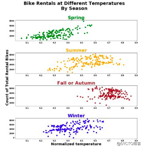
如今绘图网格重新调整,所有图的x轴都与夏天图的x轴一致(选择夏天的x轴为标准是因为它的温度范围更广)。现在可以从数据中找到一些更有趣的发现:
· 最低温度出现在春天。
· 最高温度出现在秋天。
· 在夏天和秋天,自行车租赁量和温度似乎呈二次关系。
· 不考虑季节因素时,温度越低,自行车租赁量越少。
· 春天的自行车租赁量和温度呈明显的正线性关系。
· 秋天的自行车租赁量和温度呈轻度的负线性关系。
fig = plt.figure()

plt.rcParams[‘figure.figsize‘]= [10,10]
plt.rcParams["font.weight"]= "bold"

plt.subplots_adjust(wspace=0.5)
fontdicty1={‘fontsize‘:18,
          ‘weight‘ : ‘bold‘}

fontdictx1={‘fontsize‘:18,
          ‘weight‘ : ‘bold‘,
          ‘horizontalalignment‘: ‘center‘}

fig.suptitle(‘BikeRentals at Different Temperatures\nBy Season‘,fontsize=25,fontweight="bold", color="black",
             position=(0.5,1.0))

ax3 =fig.add_subplot(143, sharey=ax3)
ax3.scatter(‘temp‘,‘cnt‘, data=day.loc[day[‘season‘]==3], c="brown")
ax3.set_title(‘Fallor Autumn‘, fontdict=fontdict,color="brown")

ax1 =fig.add_subplot(141, sharey=ax3)
ax1.scatter(‘temp‘,‘cnt‘, data=day.loc[day[‘season‘]==1], c="green")
ax1.set_title(‘Spring‘,fontdict=fontdict, color="green")
ax1.set_ylabel("Countof Total Rental Bikes", fontdict=fontdicty1, position=(0.5,0.5))

ax2 =fig.add_subplot(142, sharey=ax3)
ax2.scatter(‘temp‘,‘cnt‘, data=day.loc[day[‘season‘]==2], c="orange")
ax2.set_title(‘Summer‘,fontdict=fontdict, color="orange")

ax4 =fig.add_subplot(144, sharey=ax3)
ax4.scatter(‘temp‘,‘cnt‘, data=day.loc[day[‘season‘]==4], c="blue")
ax4.set_title(‘Winter‘,fontdict=fontdict, color="blue")
ax4.set_xlabel("Normalizedtemperature", fontdict=fontdictx, position=(-1.5,0));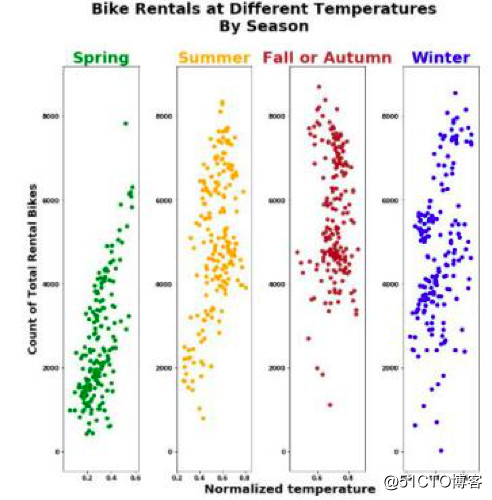
将所有绘图并列放置又有新的发现:
· 所有季节都有超过8000辆自行车出租的时间点。
· 大规模的自行车出租主要出现在春秋两季。
· 冬夏两季中自行车租赁量变动较大。
但注意,不要从以上方面来解释变量之间的关系。尽管春夏两季中自行车租赁量与气温似乎存在负线性关系,但这一解释实际是错误的。从前文的分析中我们发现事实并非如此。

seaborn包是基于Matplotlib库开发的。它用于创建更具吸引力、信息量更大的统计图形。虽然seaborn与Matplotlib不一样,但它创建的图像一样具有吸引力。
尽管matplotlib表现不俗,但我们总希望做得更好。运行下面的代码块以导入seaborn库,并创建先前的散点图,来看看会出现什么。
首先输入代码import seaborn assns,将seaborn库导入。下一行sns.set()将seaborn的默认主题和调色板加载到会话中。运行下面的代码并观察图表中哪些区域或文字发生更改。
import seaborn assns
sns.set()
将seaborn加载到会话中后,当使用Matplotlib生成图像时,这个库会添加seaborn的默认自定义项,如图所示。而最令用户感到困扰的便是它们的标题有可能会重复——Matplotlib的命名规则让人困惑,这一点也让人觉得厌烦。尽管如此,这些视觉效果依然很有吸引力,数据科学家的工作已引入这一技术。
为了使标题更加与时俱进,提高其用户友好度,需要使用如下代码。但注意,以下代码仅适用于散点图中含有副标题的情况。有的时候副标题也十分重要,因此仍需更好地掌握这种结构。
fig = plt.figure()
fig.suptitle(‘Seabornwith Python‘, fontsize=‘x-large‘, fontweight=‘bold‘)
fig.subplots_adjust(top=0.87)
#This is used forthe main title. ‘figure()‘ is a class that provides all the plotting elementsof a diagram.
#This must be usedfirst or else the title will not show.fig.subplots_adjust(top=0.85) solves ouroverlapping title problem.

ax =fig.add_subplot(111)

fontdict={‘fontsize‘:14,
        ‘fontweight‘ : ‘book‘,
        ‘verticalalignment‘: ‘baseline‘,
        ‘horizontalalignment‘: ‘center‘}

ax.set_title(‘PlottingTutorial‘, fontdict=fontdict)
#This specifieswhich plot to add the customizations. fig.add_sublpot(111) corresponds to topleft plot no.1
#(there is only oneplot).

plt.plot(x, y,‘go-‘, linewidth=1) #linewidth=1 to make it narrower
plt.xlabel(‘x-axis‘,fontsize=14)
plt.ylabel(‘yaxis‘,fontsize=14);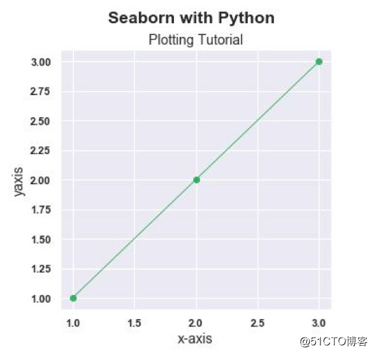
深入挖掘seaborn的功能后,我们可以用更少的代码行与类似的语法对自行车租赁量数据集再次创建可视化图。Seaborn仍然使用Matplotlib语法来生成图像,尽管新图与旧图之间的语法差异很小,但依然十分明显。
为了简化视觉效果,我们将对自行车租赁数据集的“季节”列重新命名,并重新标记。
day.rename(columns={‘season‘:‘Season‘},inplace=True)
day[‘Season‘]=day.Season.map({1:‘Spring‘,2:‘Summer‘, 3:‘Fall/Autumn‘, 4:‘Winter‘})
如今我们已根据喜好重新编辑了“季节”一栏,接下来将用seaborn对先前的绘图进行可视化。
第一个明显的区别在于——当默认样式加入到会话后,seaborn显示的默认主题不一致。上面显示的默认主题是在调用sns.set()时在后台应用sns.set_style(‘whitegrid‘)的结果。我们也可以根据喜好用已有主题改变原来的状态,如下图所示。
· sns.set_style()标记的是“white”、“dark”、“whitegrid”以及“darkgrid”中的一个。这一代码控制着整个绘图区域,比如颜色,网格以及标记的状态。
· sns.set_context()表示的是“paper”、“notebook”、“talk”和“poster”的内容。这将根据读取方式控制绘图的布局。例如,如果内容出现在“poster”上,我们将看到放大的图像和文字。如果内容出现在 “talk”中,其字体将会加粗。
plt.figure(figsize=(7,6))

fontdict={‘fontsize‘:18,
          ‘weight‘ : ‘bold‘,
         ‘horizontalalignment‘: ‘center‘}

sns.set_context(‘talk‘,font_scale=0.9)
sns.set_style(‘ticks‘)

sns.scatterplot(x=‘temp‘,y=‘cnt‘, hue=‘Season‘, data=day, style=‘Season‘,
                   palette=[‘green‘,‘orange‘,‘brown‘,‘blue‘], legend=‘full‘)

plt.legend(scatterpoints=1,
           bbox_to_anchor=(1, 0.7), loc=2,borderaxespad=1.,
           ncol=1,
           fontsize=14)
plt.xlabel(‘NormalizedTemperature‘, fontsize=16, fontweight=‘bold‘)
plt.ylabel(‘Countof Total Bike Rentals‘, fontsize=16, fontweight=‘bold‘)
plt.title(‘BikeRentals at Different Temperatures\nBy Season‘, fontdict=fontdict, color="black",
         position=(0.5,1));
现在来看一个相同的散点图,但其输入代码为sns.set_context(‘paper‘,font_scale=2)和sns.set_style(‘white‘)
plt.figure(figsize=(7,6))
fontdict={‘fontsize‘:18,
          ‘weight‘ : ‘bold‘,
         ‘horizontalalignment‘: ‘center‘}

sns.set_context(‘paper‘,font_scale=2) #this makes the font and scatterpoints much smaller, hence theneed for size adjustemnts
sns.set_style(‘white‘)

sns.scatterplot(x=‘temp‘,y=‘cnt‘, hue=‘Season‘, data=day, style=‘Season‘,
                    palette=[‘green‘,‘orange‘,‘brown‘,‘blue‘],legend=‘full‘, size=‘Season‘, sizes=[100,100,100,100])

plt.legend(scatterpoints=1,
           bbox_to_anchor=(1, 0.7), loc=2,borderaxespad=1.,
           ncol=1,
           fontsize=14)

plt.xlabel(‘NormalizedTemperature‘, fontsize=16, fontweight=‘bold‘)
plt.ylabel(‘Countof Total Bike Rentals‘, fontsize=16, fontweight=‘bold‘)
plt.title(‘BikeRentals at Different Temperatures\nBy Season‘, fontdict=fontdict,color="black",
         position=(0.5,1));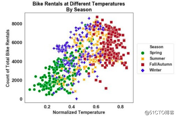
现在终于用Seaborn重新创建了之前用Matplotlib生成的散点图。更改后的图使用的代码行数更少,分辨率也更高。接下来继续完成绘图:
sns.set(rc={‘figure.figsize‘:(20,20)})
sns.set_context(‘talk‘,font_scale=2)
sns.set_style(‘ticks‘)
g =sns.relplot(x=‘temp‘, y=‘cnt‘, hue=‘Season‘, data=day,palette=[‘green‘,‘orange‘,‘brown‘,‘blue‘],
                col=‘Season‘, col_wrap=4,legend=False
                height=6, aspect=0.5,style=‘Season‘, sizes=(800,1000))

g.fig.suptitle(‘BikeRentals at Different Temperatures\nBy Season‘ ,position=(0.5,1.05),fontweight=‘bold‘, size=18)
g.set_xlabels("NormalizedTemperature",fontweight=‘bold‘, size=15)
g.set_ylabels("Countof Total Bike Rentals",fontweight=‘bold‘, size=20);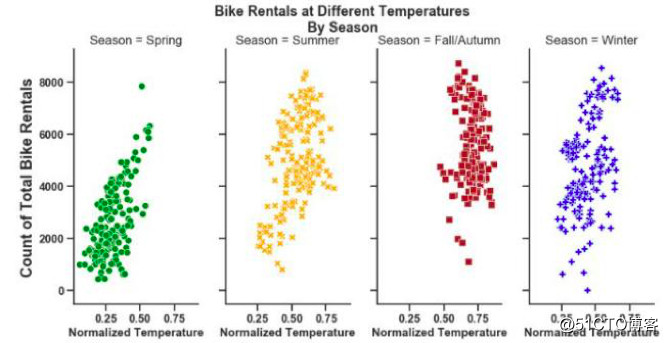
改变图表形状需要改变外观参数。通过增大外观的数值,图表形状会更呈方形。图像高度也会随着数值更改发生变化,因此这里需要同时对两个参数进行试验。
更改行数和列数需使用col_wrap参数执行此操作。行数和列数会随着col参数而变化。这种参数可以检测类比数目,同时可以相应地分配。
sns.set(rc={‘figure.figsize‘:(20,20)})
sns.set_context(‘talk‘,font_scale=2)
sns.set_style(‘ticks‘)
g =sns.relplot(x=‘temp‘, y=‘cnt‘, hue=‘Season‘,data=day,palette=[‘green‘,‘orange‘,‘brown‘,‘blue‘],
                col=‘Season‘, col_wrap=2,legend=False
                height=4, aspect=1.6,style=‘Season‘, sizes=(800,1000))

g.fig.suptitle(‘BikeRentals at Different Temperatures\nBy Season‘ ,position=(0.5,1.05),fontweight=‘bold‘, size=18)
g.set_xlabels("NormalizedTemperature",fontweight=‘bold‘, size=15)
g.set_ylabels("Countof\nTotal Bike Rentals",fontweight=‘bold‘, size=20);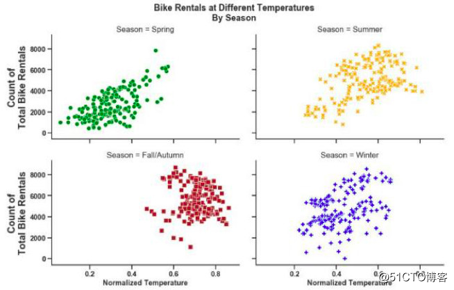
编译组:伍颖欣、李美欣
相关链接:
https://www.kdnuggets.com/2019/04/data-visualization-python-matplotlib-seaborn.html

如需转载,请后台留言,遵守转载规范ACL2018论文集50篇解读
EMNLP2017论文集28篇论文解读
2018年AI三大顶会中国学术成果全链接
ACL2017 论文集:34篇解读干货全在这里
10篇AAAI2017经典论文回顾
Matplotlib+Seaborn:一文掌握Python可视化库的两大王者
标签:经典 fonts wrap 朋友 ipy 有趣 隐藏 style pad
原文地址:https://blog.51cto.com/15057819/2567648