创建一个Caffe model，你需要在一个prototxt（protocol buffer definition file）文件中定义一个模型结构。

caffe的层结构和参数被定义在caffe.proto文件中。

Header: ./include/caffe/vision_layers.hpp

          可视层一般将图片作为输入然后产生其他类型的图片作为输出。一个典型‘images‘(图片)在真实的世界可能只有一个颜色通道（c=1）,作为一张灰度图，或者三个颜色通道（c=3）,作为RGB（红、绿、蓝）图像。但是在这篇文章中，图像的特征是他的结构空间：通常情况一张图片有一些non-trivial高度h>1和宽度w>1。这种二维几何构造明确了如何处理输入（intput）。特别是，大多数的可视层的工作，是通过施加特定的操作在输入图片的一些区域，以产生相应的输出区域。相比之下，其他层忽略输入的空间结构，把他认为是一个“one big vector”用c、h、w三个维度表示。

层类型：卷积层

CPU接口：./src/caffe/layers/convolution_layer.cpp

CUDA GPU接口：./src/caffe/layers/convolution_layer.cu

参数：

    必须有的参数：

                    num_output (c_o): the number of filters      //卷积核的个数

                    kernel_size (or kernel_h and kernel_w): specifies height and width of each filter    //每一个卷积核的高和宽

     

     强烈推荐的参数：

                     weight_filler [default type: ‘constant‘ value: 0]   //初始化kernel，参数的初始化方法

     可选的参数：

                    bias_term [default true]: 指定是否学习和应用一系列偏置
                   pad (or pad_h and pad_w) [default 0]: 指定在输入的每一边加上多少个像素
                  stride (or stride_h and stride_w) [default 1]:指定过滤器kernel的步长
                  group (g) [default 1]: If g > 1, 将输入的特征图进行分组操作，我们限制每个过滤器的连接到一个子集的输入。具体来说，输入和输出通道分为G组，第i个输出组只能连接到第i个输入组。

输入：

      n * c_i * h_i * w_i

输出：

       n * c_o * h_o * w_o, where h_o = (h_i + 2 * pad_h - kernel_h) / stride_h + 1 and w_o likewise.  

案例：            

      layer {
  name: "conv1"
  type: "Convolution"
  bottom: "data"
  top: "conv1"
  # learning rate and decay multipliers for the filters
  param { lr_mult: 1 decay_mult: 1 }
  # learning rate and decay multipliers for the biases
  param { lr_mult: 2 decay_mult: 0 }
  convolution_param {
    num_output: 96     # learn 96 filters
    kernel_size: 11    # each filter is 11x11
    stride: 4          # step 4 pixels between each filter application
    weight_filler {
      type: "gaussian" # initialize the filters from a Gaussian
      std: 0.01        # distribution with stdev 0.01 (default mean: 0)
    }
    bias_filler {
      type: "constant" # initialize the biases to zero (0)
      value: 0
    }
  }
}

卷积层：让输入图片和一系列可学习的过滤器进行卷积，每一个过滤器卷积完全图后产生一个特征图（feature map）

1.2 Pooling（池化层）

       n * c * h_i * w_i

输出：
       n * c_o * h_o * w_o, where h_o = (h_i + 2 * pad_h - kernel_h) / stride_h + 1 and w_o likewise.  

案例：

layer {
  name: "pool1"
  type: "Pooling"
  bottom: "conv1"
  top: "pool1"
  pooling_param {
    pool: MAX
    kernel_size: 3 # pool over a 3x3 region
    stride: 2      # step two pixels (in the bottom blob) between pooling regions
  }
}

1.3 Local Response Normalization (LRN)

层类型：LRN

CPU接口：./src/caffe/layers/lrn_layer.cpp

GPU接口：./src/caffe/layers/lrn_layer.cu

参数：

    可选参数：

         local_size [default 5]：对于cross channel LRN为需要求和的邻近channel的数量；对于within channel LRN为需要求和的空间区域的边长
         alpha [default 1]：scaling参数
         beta [default 5]：指数
         norm_region [default ACROSS_CHANNELS]: 选择哪种LRN的方法ACROSS_CHANNELS 或者WITHIN_CHANNEL

         Local ResponseNormalization是对一个局部的输入区域进行的归一化（激活a被加一个归一化权重（分母部分）生成了新的激活b），有两种不同的形式，一种的输入区域为相邻的channels（cross channel LRN），另一种是为同一个channel内的空间区域（within channel LRN）


计算公式：对每一个输入除以

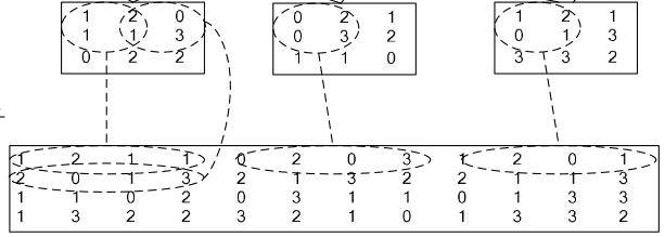
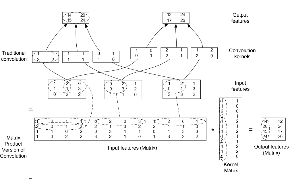
如果对matlab比较熟悉的话，就应该知道im2col是什么意思。它先将一个大矩阵，重叠地划分为多个子矩阵，对每个子矩阵序列化成向量，最后得到另外一个矩阵。

在caffe中，卷积运算就是先对数据进行im2col操作，再进行内积运算（inner product)。这样做，比原始的卷积操作速度更快。


看看两种卷积操作的异同：

深度学习是通过最小化输出和目标的Loss来驱动学习

层类型：SoftmaxWithLoss

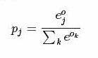
softmax-loss层和softmax层计算大致是相同的softmax是一个分类器，计算的是类别的概率（Likelihood），是Logistic Regression 的一种推广。Logistic Regression 只能用于二分类，而softmax可以用于多分类。

softmax计算公式：。

layer {
  name: "loss"
  type: "SoftmaxWithLoss"
  bottom: "ip1"
  bottom: "label"
  top: "loss"
}

softmax layer: 输出似然值

layers {
  bottom: "cls3_fc"
  top: "prob"
  name: "prob"
  type: “Softmax"
}

2.2 Sum-of-Squares/Euclidean
2.3 Hinge/Margin
2.4 sigmoid Cross-Entropy
2.5 Infogain
2.6Accuracy and Top-k

3 Activation/Neuron Layers(激活层)

输入：n*c*h*w

输出：n*c*h*w

layer {
  name: "encode1neuron"
  bottom: "encode1"
  top: "encode1neuron"
  type: "Sigmoid"
}

3.2 ReLU / Rectified-Linear and Leaky-ReLU

ReLU是目前使用最多的激活函数，主要因为其收敛更快，并且能保持同样效果

layer {
  name: "relu1"
  type: "ReLU"
  bottom: "pool1"
  top: "pool1"
}

RELU层支持in-place计算，这意味着bottom的输出和输入相同以避免内存的消耗。

3.3 TanH / Hyperbolic Tangent

利用双曲正切函数对数据进行变换。

层类型：TanH
layer {
  name: "layer"
  bottom: "in"
  top: "out"
  type: "TanH"
}

3.4、Absolute Value

求每个输入数据的绝对值。
f(x)=Abs(x)
层类型：AbsVal
layer {
  name: "layer"
  bottom: "in"
  top: "out"
  type: "AbsVal"
}

3.5、Power

对每个输入数据进行幂运算
f(x)= (shift + scale * x) ^ power
层类型：Power
可选参数：
　　power: 默认为1
　　scale: 默认为1
　　shift: 默认为0
layer {
  name: "layer"
  bottom: "in"
  top: "out"
  type: "Power"
  power_param {
    power: 2
    scale: 1
    shift: 0
  }
}

3.6、BNLL

binomial normal log likelihood的简称
f(x)=log(1 + exp(x))
层类型：BNLL
layer {
  name: "layer"
  bottom: "in"
  top: "out"
  type: “BNLL”
}

4 data layers

5 Common Layers

5.1 Inner Product

全连接层，把输入当作成一个向量，输出也是一个简单向量（把输入数据blobs的width和height全变为1）。
输入： n*c0*h*w
输出： n*c1*1*1
全连接层实际上也是一种卷积层，只是它的卷积核大小和原数据大小一致。因此它的参数基本和卷积层的参数一样。
层类型：InnerProduct
lr_mult: 学习率的系数，最终的学习率是这个数乘以solver.prototxt配置文件中的base_lr。如果有两个lr_mult, 则第一个表示权值的学习率，第二个表示偏置项的学习率。一般偏置项的学习率是权值学习率的两倍。
必须设置的参数：
  　　num_output: 过滤器（filfter)的个数
其它参数：
    　　weight_filler: 权值初始化。 默认为“constant",值全为0，很多时候我们用"xavier"算法来进行初始化，也可以设置为”gaussian"
    　　bias_filler: 偏置项的初始化。一般设置为"constant",值全为0。
   　　 bias_term: 是否开启偏置项，默认为true, 开启
layer {
  name: "ip1"
  type: "InnerProduct"
  bottom: "pool2"
  top: "ip1"
  param {
    lr_mult: 1
  }
  param {
    lr_mult: 2
  }
  inner_product_param {
    num_output: 500
    weight_filler {
      type: "xavier"
    }
    bias_filler {
      type: "constant"
    }
  }
}

5.2 accuracy

输出分类（预测）精确度，只有test阶段才有，因此需要加入include参数。
层类型：Accuracy
layer {
  name: "accuracy"
  type: "Accuracy"
  bottom: "ip2"
  bottom: "label"
  top: "accuracy"
  include {
    phase: TEST
  }
}

5.3、reshape

在不改变数据的情况下，改变输入的维度。
层类型：Reshape
先来看例子
 layer {
    name: "reshape"
    type: "Reshape"
    bottom: "input"
    top: "output"
    reshape_param {
      shape {
        dim: 0  # copy the dimension from below
        dim: 2
        dim: 3
        dim: -1 # infer it from the other dimensions
      }
    }
  }

有一个可选的参数组shape, 用于指定blob数据的各维的值（blob是一个四维的数据：n*c*w*h）。

dim:0  表示维度不变，即输入和输出是相同的维度。
dim:2 或 dim:3 将原来的维度变成2或3
dim:-1 表示由系统自动计算维度。数据的总量不变，系统会根据blob数据的其它三维来自动计算当前维的维度值 。
假设原数据为：64*3*28*28， 表示64张3通道的28*28的彩色图片
经过reshape变换：
   reshape_param {
      shape {
        dim: 0 
        dim: 0
        dim: 14
        dim: -1 
      }
    }

输出数据为：64*3*14*56

5.4 Dropout

Dropout是一个防止过拟合的trick。可以随机让网络某些隐含层节点的权重不工作。
先看例子：
layer {
  name: "drop7"
  type: "Dropout"
  bottom: "fc7-conv"
  top: "fc7-conv"
  dropout_param {
    dropout_ratio: 0.5
  }
}
只需要设置一个dropout_ratio就可以了。
还有其它更多的层，但用的地方不多，就不一一介绍了。
随着深度学习的深入，各种各样的新模型会不断的出现，因此对应的各种新类型的层也在不断的出现。这些新出现的层，我们只有在等caffe更新到新版本后，再去慢慢地摸索了。