标签:
第一行:代码中的numpy是matlab的矩阵运算工具箱。Python在通过import命令加载numpy工具箱后就可以像matlab一样工作了。
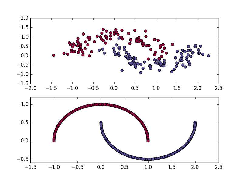
subplot(2,1,1)是噪声为0.2的数据(上部),subplot(2,1,2)是噪声为0的数据(下部)
def call_clf_predict(x):plot_decision_boundary(call_clf_predict)
# Generate a dataset and plot it(x-algo.cn)
import numpy as np
import sklearn
import sklearn.datasets
import matplotlib.pyplot as plt
import sklearn.linear_model
# Helper function to plot a decision boundary.
# If you don‘t fully understand this function don‘t worry, it just generates the contour plot below.
def plot_decision_boundary(pred_func):
# Set min and max values and give it some padding
x_min, x_max = X[:, 0].min() - .5, X[:, 0].max() + .5
y_min, y_max = X[:, 1].min() - .5, X[:, 1].max() + .5
h = 0.01
# Generate a grid of points with distance h between them
xx, yy = np.meshgrid(np.arange(x_min, x_max, h), np.arange(y_min, y_max, h))
# Predict the function value for the whole gid
Z = pred_func(np.c_[xx.ravel(), yy.ravel()])
Z = Z.reshape(xx.shape)
# Plot the contour and training examples
plt.contourf(xx, yy, Z, cmap=plt.cm.Spectral)
plt.scatter(X[:, 0], X[:, 1], c=y, cmap=plt.cm.Spectral)
# Helper function to evaluate the total loss on the dataset
def calculate_loss(model):
W1, b1, W2, b2 = model[‘W1‘], model[‘b1‘], model[‘W2‘], model[‘b2‘]
# Forward propagation to calculate our predictions
z1 = X.dot(W1) + b1
a1 = np.tanh(z1)
z2 = a1.dot(W2) + b2
exp_scores = np.exp(z2)
probs = exp_scores / np.sum(exp_scores, axis=1, keepdims=True)
# Calculating the loss
corect_logprobs = -np.log(probs[range(num_examples), y])
data_loss = np.sum(corect_logprobs)
# Add regulatization term to loss (optional)
data_loss += reg_lambda/2 * (np.sum(np.square(W1)) + np.sum(np.square(W2)))
return 1./num_examples * data_loss
# Helper function to predict an output (0 or 1)
def predict(model, x):
W1, b1, W2, b2 = model[‘W1‘], model[‘b1‘], model[‘W2‘], model[‘b2‘]
# Forward propagation
z1 = x.dot(W1) + b1
a1 = np.tanh(z1)
z2 = a1.dot(W2) + b2
exp_scores = np.exp(z2)
probs = exp_scores / np.sum(exp_scores, axis=1, keepdims=True)
return np.argmax(probs, axis=1)
# This function learns parameters for the neural network and returns the model.
# - nn_hdim: Number of nodes in the hidden layer
# - num_passes: Number of passes through the training data for gradient descent
# - print_loss: If True, print the loss every 1000 iterations
def build_model(nn_hdim, num_passes=20000, print_loss=False):
# Initialize the parameters to random values. We need to learn these.
np.random.seed(0)
W1 = np.random.randn(nn_input_dim, nn_hdim) / np.sqrt(nn_input_dim)
b1 = np.zeros((1, nn_hdim))
W2 = np.random.randn(nn_hdim, nn_output_dim) / np.sqrt(nn_hdim)
b2 = np.zeros((1, nn_output_dim))
# This is what we return at the end
model = {}
# Gradient descent. For each batch...
for i in xrange(0, num_passes):
# Forward propagation
z1 = X.dot(W1) + b1
a1 = np.tanh(z1)
z2 = a1.dot(W2) + b2
exp_scores = np.exp(z2)
probs = exp_scores / np.sum(exp_scores, axis=1, keepdims=True)
# Backpropagation
delta3 = probs
delta3[range(num_examples), y] -= 1
dW2 = (a1.T).dot(delta3)
db2 = np.sum(delta3, axis=0, keepdims=True)
delta2 = delta3.dot(W2.T) * (1 - np.power(a1, 2))
dW1 = np.dot(X.T, delta2)
db1 = np.sum(delta2, axis=0)
# Add regularization terms (b1 and b2 don‘t have regularization terms)
dW2 += reg_lambda * W2
dW1 += reg_lambda * W1
# Gradient descent parameter update
W1 += -epsilon * dW1
b1 += -epsilon * db1
W2 += -epsilon * dW2
b2 += -epsilon * db2
# Assign new parameters to the model
model = { ‘W1‘: W1, ‘b1‘: b1, ‘W2‘: W2, ‘b2‘: b2}
# Optionally print the loss.
# This is expensive because it uses the whole dataset, so we don‘t want to do it too often.
if print_loss and i % 1000 == 0:
print "Loss after iteration %i: %f" %(i, calculate_loss(model))
return model
np.random.seed(0)
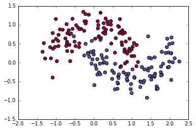
X, y = sklearn.datasets.make_moons(200, noise=0.20)
plt.scatter(X[:,0], X[:,1], s=40, c=y, cmap=plt.cm.Spectral)
clf = sklearn.linear_model.LogisticRegressionCV()
clf.fit(X, y)
num_examples = len(X) # training set size
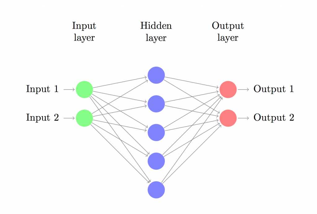
nn_input_dim = 2 # input layer dimensionality
nn_output_dim = 2 # output layer dimensionality
# Gradient descent parameters (I picked these by hand)
epsilon = 0.01 # learning rate for gradient descent
reg_lambda = 0.01 # regularization strength
# Build a model with a 3-dimensional hidden layer
model = build_model(3, print_loss=True)
# Plot the decision boundary
plot_decision_boundary(lambda x: predict(model, x))
plt.title("Decision Boundary for hidden layer size 3")
plt.show()
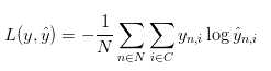
这个公式看起来比较复杂,他其实最终的意思就是统计一下有多少个预测标签ybar和y不太一样。其次要解决的就是梯度下降算法所应用的目标。在这里,分别需要用L对W1,W2,b1,b2求偏导数,结果如下所示:
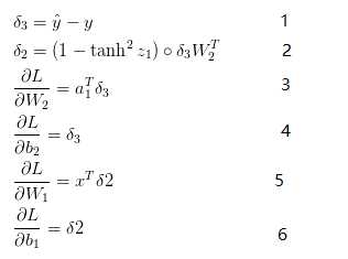
上方的最后四个式子就是L函数在W1,W2,b1,b2四个方向的梯度。
标签:
原文地址:http://www.cnblogs.com/hdu-zsk/p/5951428.html