标签:color 示例 nal lte his with nbsp markers unit
代码:
%% ------------------------------------------------------------------------
%%            Output Info about this m-file
fprintf(‘\n***********************************************************\n‘);
fprintf(‘        <DSP using MATLAB> Exameple 9.10 \n\n‘);

time_stamp = datestr(now, 31);
[wkd1, wkd2] = weekday(today, ‘long‘);
fprintf(‘      Now is %20s, and it is %7s  \n\n‘, time_stamp, wkd2);
%% ------------------------------------------------------------------------

% Given parameters:
n = [0:50]; wxp = 0.5*pi; x = cos(wxp*n);
n1 = n(1:9); x1 = x(9:17);             % for plotting purposes

I = 5; Rp = 0.01; As = 50; wp = wxp/I; ws = (2*pi-wxp)/I;
[delta1, delta2] = db2delta(Rp, As); weights = [delta2/delta1, 1];
[N, Fo, Ao, weights] = firpmord([wp, ws]/pi, [1, 0], [delta1, delta2], 2); N = N + 2;
N

%% -----------------------------------------------------------------
%%                             Plot
%% -----------------------------------------------------------------

% Input signal
Hf1 = figure(‘units‘, ‘inches‘, ‘position‘, [1, 1, 8, 6], ...
	‘paperunits‘, ‘inches‘, ‘paperposition‘, [0, 0, 6, 4], ...
	‘NumberTitle‘, ‘off‘, ‘Name‘, ‘Exameple 9.10‘);
set(gcf,‘Color‘,‘white‘);

TF = 10;

subplot(2, 2, 1);
Hs1 = stem(n1, x1, ‘filled‘); set(Hs1, ‘markersize‘, 2, ‘color‘, ‘g‘);
axis([-1, 9, -1.2, 1.2]); grid on;
xlabel(‘n‘, ‘vertical‘, ‘middle‘); ylabel(‘Amplitude‘);
title(‘Input Signal x(n)‘, ‘fontsize‘, TF);
set(gca, ‘xtick‘, [0:4:16]);
set(gca, ‘ytick‘, [-1, 0, 1]);


% Interpolation with Filter Design: Length M=31
%M = 31; F = [0, wp, ws, pi]/pi; A = [I, I, 0, 0];
h = firpm(N, Fo, I*Ao, weights); y = upfirdn(x, h, I);
delay = (N)/2;                                                   % Delay imparted by the filter
m = delay+1:1:50*I+delay+1; y = y(m); m = 0:40; y = y(81:121);   % for plotting


subplot(2, 2, 3);
Hs2 = stem(m, y, ‘filled‘); axis([-5, 45, -1.2, 1.2]); grid on;
set(Hs2, ‘markersize‘, 2, ‘color‘, ‘m‘);
xlabel(‘m‘, ‘vertical‘, ‘middle‘); ylabel(‘Amplitude‘);
title(‘ Output Singal y(n): I = 5‘, ‘fontsize‘, TF);
set(gca, ‘xtick‘, [0:4:16]*I);
set(gca, ‘ytick‘, [-1, 0, 1]);


% Filter Desing Plots
[Hr, w, a, L] = Hr_Type1(h); Hr_min = min(Hr); w_min = find(Hr == Hr_min);
H = abs(freqz(h, 1, w)); Hdb = 20*log10(H/max(H)); min_attn = Hdb(w_min);

subplot(2, 2, 2);
plot(w/pi, Hr, ‘m‘, ‘linewidth‘, 1.0); axis([0, 1, -1, 6]); grid on;
xlabel(‘Frequency in \pi units‘, ‘vertical‘, ‘middle‘); ylabel(‘Amplitude‘);
title(‘Amplitude Response ‘, ‘fontsize‘, TF);
set(gca, ‘xtick‘, [0, wp/pi, ws/pi, 1]);
set(gca, ‘ytick‘, [0, I]);

subplot(2, 2, 4);
plot(w/pi, Hdb, ‘m‘, ‘linewidth‘, 1.0); axis([0, 1, -70, 10]); grid on;
xlabel(‘Frequency in \pi units‘, ‘vertical‘, ‘middle‘); ylabel(‘Decibels‘);
title(‘Log-magnitude Response ‘, ‘fontsize‘, TF);
set(gca, ‘xtick‘, [0, wp/pi, ws/pi, 1]);
set(gca, ‘ytick‘, [-70, round(min_attn), 0]);
运行结果:
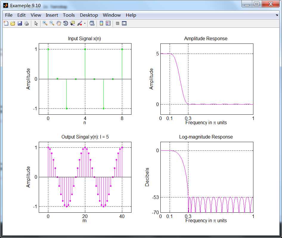
设计的滤波器最小阻带衰减为53dB。
《DSP using MATLAB》示例 Example 9.10
标签:color 示例 nal lte his with nbsp markers unit
原文地址:http://www.cnblogs.com/ky027wh-sx/p/6913396.html