机器学习中的预测问题通常分为2类：回归与分类

标签：0.00   归类   RoCE   process   red   new   proc   res   预测   

回归就是预测数值，而分类是给数据打上标签归类。

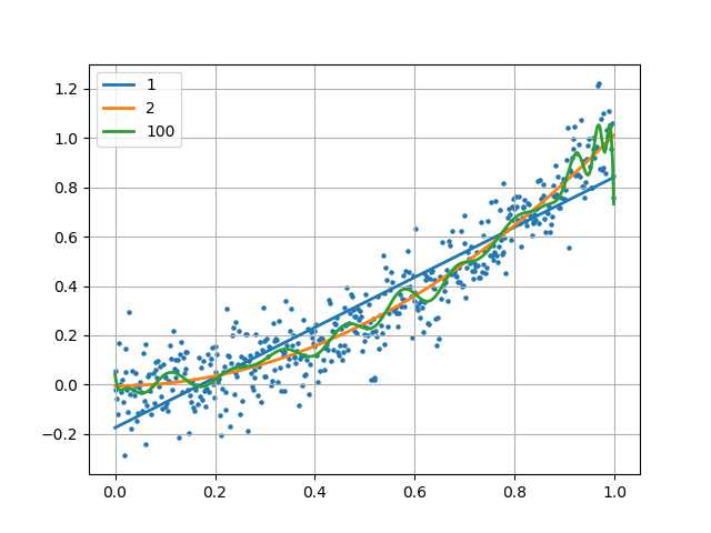
本例中使用一个2次函数加上随机的扰动来生成500个点，然后尝试用1、2、100次方的多项式对该数据进行拟合。

拟合的目的是使得根据训练数据能够拟合出一个多项式函数，这个函数能够很好的拟合现有数据，并且能对未知的数据进行预测。

import matplotlib.pyplot as plt
import numpy as np
import scipy as sp
from scipy.stats import norm
from sklearn.pipeline import Pipeline
from sklearn.linear_model import LinearRegression
from sklearn.preprocessing import PolynomialFeatures
from sklearn import linear_model

‘‘‘ 数据生成 ‘‘‘
x = np.arange(0, 1, 0.002)
y = norm.rvs(0, size=500, scale=0.1)
y = y + x**2

‘‘‘ 均方误差根 ‘‘‘
def rmse(y_test, y):
    return sp.sqrt(sp.mean((y_test - y) ** 2))

‘‘‘ 与均值相比的优秀程度，介于[0~1]。0表示不如均值。1表示完美预测.这个版本的实现是参考scikit-learn官网文档  ‘‘‘
def R2(y_test, y_true):
    return 1 - ((y_test - y_true)**2).sum() / ((y_true - y_true.mean())**2).sum()


‘‘‘ 这是Conway&White《机器学习使用案例解析》里的版本 ‘‘‘
def R22(y_test, y_true):
    y_mean = np.array(y_true)
    y_mean[:] = y_mean.mean()
    return 1 - rmse(y_test, y_true) / rmse(y_mean, y_true)


plt.scatter(x, y, s=5)
degree = [1,2,100]
y_test = []
y_test = np.array(y_test)


for d in degree:
    clf = Pipeline([(‘poly‘, PolynomialFeatures(degree=d)),(‘linear‘, LinearRegression(fit_intercept=False))])
    clf.fit(x[:, np.newaxis], y)
    y_test = clf.predict(x[:, np.newaxis])

    print(clf.named_steps[‘linear‘].coef_)
    print(‘rmse=%.2f, R2=%.2f, R22=%.2f, clf.score=%.2f‘%
          (rmse(y_test, y),R2(y_test, y), R22(y_test, y),
           clf.score(x[:, np.newaxis], y)))
    plt.plot(x, y_test, linewidth=2)
plt.grid()
plt.legend([‘1‘,‘2‘,‘100‘], loc=‘upper left‘)
plt.show()

 原文出处：https://blog.csdn.net/lsldd/article/details/41251583（转载）

机器学习中的预测问题通常分为2类：回归与分类

标签：0.00   归类   RoCE   process   red   new   proc   res   预测   

原文地址：https://www.cnblogs.com/heaiping/p/9067977.html