标签：tor   pretty   erro   --   model   b2c   tar   epo   []   

from __future__ import division, print_function, absolute_import

import tflearn
import numpy as np
import math
import matplotlib
matplotlib.use(‘Agg‘)
import matplotlib.pyplot as plt
import tensorflow as tf

step_radians = 0.001
steps_of_history = 10
steps_in_future = 5
learning_rate = 0.003

def getData(x):
    seq = []
    next_val = []
    for i in range(0, len(x) - steps_of_history - steps_in_future, steps_in_future):
        seq.append(x[i: i + steps_of_history])
        next_val.append(x[i + steps_of_history + steps_in_future -1])
    
    seq = np.reshape(seq, [-1, steps_of_history, 1])
    next_val = np.reshape(next_val, [-1, 1])
    X = np.array(seq)
    Y = np.array(next_val)
    return X,Y

def myRNN(activator,optimizer):
    tf.reset_default_graph()
    # Network building
    net = tflearn.input_data(shape=[None, steps_of_history, 1])
    net = tflearn.lstm(net, 32, dropout=0.8,bias=True)
    net = tflearn.fully_connected(net, 1, activation=activator)
    net = tflearn.regression(net, optimizer=optimizer, loss=‘mean_square‘, learning_rate=learning_rate)
    
    # Training Data
    trainVal = np.sin(np.arange(0, 20*math.pi, step_radians))
    trainX,trainY = getData(trainVal)
    print(np.shape(trainX))
    
    # Training
    model = tflearn.DNN(net)
    model.fit(trainX, trainY, n_epoch=10, validation_set=0.1, batch_size=128)
    
    # Testing Data
    testVal = np.sin(np.arange(20*math.pi, 24*math.pi, step_radians))
    testX,testY = getData(testVal)
    
    # Predict the future values
    predictY = model.predict(testX)
    
    print("---------TEST ERROR-----------")
    expected = np.array(testY).flatten()
    predicted = np.array(predictY).flatten()
    error = sum(((expected - predicted) **2)/len(expected))
    print(error)
    
    # Plot and save figure
    plotFig(testY, np.array(predictY).flatten(), error, activator+"_"+optimizer)

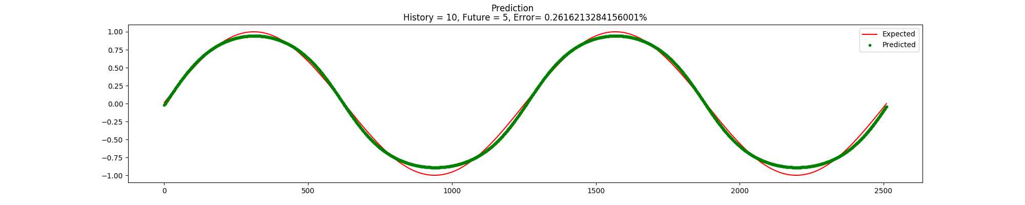
def plotFig(actual,predicted,error,filename):
    # Plot the results
    plt.figure(figsize=(20,4))
    plt.suptitle(‘Prediction‘)
    plt.title(‘History = ‘+str(steps_of_history)+‘, Future = ‘+str(steps_in_future)+‘, Error= ‘+str(error*100)+‘%‘)
    plt.plot(actual, ‘r-‘, label=‘Expected‘)
    plt.plot(predicted, ‘g.‘, label=‘Predicted‘)
    plt.legend()
    plt.savefig(filename+‘.png‘)
    
def main():
    activators = [‘linear‘, ‘tanh‘, ‘sigmoid‘, ‘softmax‘, ‘softplus‘, ‘softsign‘, ‘relu‘, ‘relu6‘, ‘leaky_relu‘, ‘prelu‘, ‘elu‘]
    optimizers = [‘sgd‘, ‘rmsprop‘, ‘adam‘, ‘momentum‘, ‘adagrad‘, ‘ftrl‘, ‘adadelta‘]
    for activator in activators:    
        for optimizer in optimizers:
            print ("Running for : "+ activator + " & " + optimizer)
            myRNN(activator, optimizer)
            break
        break

main()

 效果：

其他参考代码：

# Simple example using recurrent neural network to predict time series values

from __future__ import division, print_function, absolute_import

import tflearn
from tflearn.layers.normalization import batch_normalization
import numpy as np
import math
import matplotlib
matplotlib.use(‘Agg‘)
import matplotlib.pyplot as plt

step_radians = 0.01
steps_of_history = 200
steps_in_future = 1
index = 0

x = np.sin(np.arange(0, 20*math.pi, step_radians))

seq = []
next_val = []

for i in range(0, len(x) - steps_of_history, steps_in_future):
    seq.append(x[i: i + steps_of_history])
    next_val.append(x[i + steps_of_history])

seq = np.reshape(seq, [-1, steps_of_history, 1])
next_val = np.reshape(next_val, [-1, 1])
print(np.shape(seq))

trainX = np.array(seq)
trainY = np.array(next_val)

# Network building
net = tflearn.input_data(shape=[None, steps_of_history, 1])
net = tflearn.simple_rnn(net, n_units=32, return_seq=False)
net = tflearn.fully_connected(net, 1, activation=‘linear‘)
net = tflearn.regression(net, optimizer=‘sgd‘, loss=‘mean_square‘, learning_rate=0.1)

# Training
model = tflearn.DNN(net, clip_gradients=0.0, tensorboard_verbose=0)
model.fit(trainX, trainY, n_epoch=15, validation_set=0.1, batch_size=128)

# Testing
x = np.sin(np.arange(20*math.pi, 24*math.pi, step_radians))

seq = []

for i in range(0, len(x) - steps_of_history, steps_in_future):
    seq.append(x[i: i + steps_of_history])

seq = np.reshape(seq, [-1, steps_of_history, 1])
testX = np.array(seq)

# Predict the future values
predictY = model.predict(testX)
print(predictY)

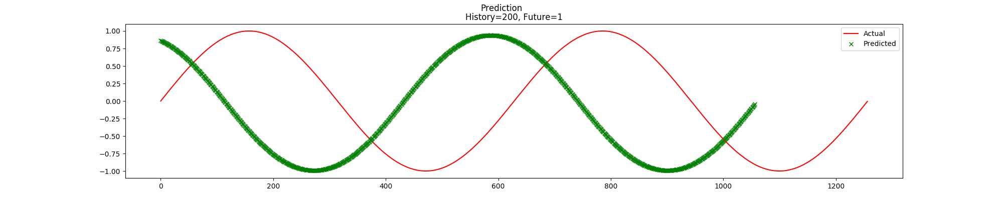
# Plot the results
plt.figure(figsize=(20,4))
plt.suptitle(‘Prediction‘)
plt.title(‘History=‘+str(steps_of_history)+‘, Future=‘+str(steps_in_future))
plt.plot(x, ‘r-‘, label=‘Actual‘)
plt.plot(predictY, ‘gx‘, label=‘Predicted‘)
plt.legend()
plt.savefig(‘sine.png‘)

 效果：

参考：

https://github.com/tflearn/tflearn/issues/121

https://mourafiq.com/2016/05/15/predicting-sequences-using-rnn-in-tensorflow.html

https://blog.csdn.net/weiwei9363/article/details/78904383

摘录tensorflow处理的做法：

RNN - 预测正弦函数

• 参考《TensorFlow实战Google深度学习框架》。不使用TFLearn，只使用TensorFlow
• 完整代码看这里
• 如果对RNN不理解，请看RNN递归神经网络的直观理解：基于TensorFlow的简单RNN例子

import tensorflow as tf
import numpy as np
import matplotlib.pyplot as plt
%matplotlib inline

数据准备

# 训练数据个数
training_examples = 10000
# 测试数据个数
testing_examples = 1000
# sin函数的采样间隔
sample_gap = 0.01
# 每个训练样本的长度
timesteps = 20

def generate_data(seq):
    ‘‘‘
    生成数据，seq是一序列的连续的sin的值
    ‘‘‘
    X = []
    y = []

    # 用前 timesteps 个sin值，估计第 timesteps+1 个
    # 因此， 输入 X 是一段序列，输出 y 是一个值 
    for i in range(len(seq) - timesteps -1):
        X.append(seq[i : i+timesteps])
        y.append(seq[i+timesteps])

    return np.array(X, dtype=np.float32), np.array(y, dtype=np.float32)

test_start = training_examples*sample_gap
test_end = test_start + testing_examples*sample_gap

train_x, train_y = generate_data( np.sin( np.linspace(0, test_start, training_examples) ) )
test_x, test_y = generate_data( np.sin( np.linspace(test_start, test_end, testing_examples) ) )

建立RNN模型

设置模型参数

lstm_size = 30
lstm_layers = 2
batch_size = 64

定义输入输出

x = tf.placeholder(tf.float32, [None, timesteps, 1], name=‘input_x‘)
y_ = tf.placeholder(tf.float32, [None, 1], name=‘input_y‘)
keep_prob = tf.placeholder(tf.float32, name=‘keep_prob‘)

建立LSTM层

# 有lstm_size个单元
lstm = tf.contrib.rnn.BasicLSTMCell(lstm_size)
# 添加dropout
drop = tf.contrib.rnn.DropoutWrapper(lstm, output_keep_prob=keep_prob)
# 一层不够，就多来几层
def lstm_cell():
    return tf.contrib.rnn.BasicLSTMCell(lstm_size)
cell = tf.contrib.rnn.MultiRNNCell([ lstm_cell() for _ in range(lstm_layers)])

# 进行forward，得到隐层的输出
outputs, final_state = tf.nn.dynamic_rnn(cell, x, dtype=tf.float32)
# 在本问题中只关注最后一个时刻的输出结果，该结果为下一个时刻的预测值
outputs = outputs[:,-1]

# 定义输出层, 输出值[-1,1]，因此激活函数用tanh
predictions = tf.contrib.layers.fully_connected(outputs, 1, activation_fn=tf.tanh)
# 定义损失函数
cost = tf.losses.mean_squared_error(y_, predictions)
# 定义优化步骤
optimizer = tf.train.AdamOptimizer().minimize(cost)

训练

# 获取一个batch_size大小的数据
def get_batches(X, y, batch_size=64):
    for i in range(0, len(X), batch_size):
        begin_i = i
        end_i = i + batch_size if (i+batch_size) < len(X) else len(X)

        yield X[begin_i:end_i], y[begin_i:end_i]

epochs = 20
session = tf.Session()
with session.as_default() as sess:
    # 初始化变量
    tf.global_variables_initializer().run()

    iteration = 1

    for e in range(epochs):
        for xs, ys in get_batches(train_x, train_y, batch_size):
            # xs[:,:,None] 增加一个维度，例如[64, 20] ==> [64, 20, 1]，为了对应输入
            # 同理 ys[:,None]
            feed_dict = { x:xs[:,:,None], y_:ys[:,None], keep_prob:.5 }

            loss, _ = sess.run([cost, optimizer], feed_dict=feed_dict)

            if iteration % 100 == 0:
                print(‘Epochs:{}/{}‘.format(e, epochs),
                      ‘Iteration:{}‘.format(iteration),
                      ‘Train loss: {:.8f}‘.format(loss))
            iteration += 1

Epochs:0/20 Iteration:100 Train loss: 0.01009926
Epochs:1/20 Iteration:200 Train loss: 0.02012673
Epochs:1/20 Iteration:300 Train loss: 0.00237983
Epochs:2/20 Iteration:400 Train loss: 0.00029798
Epochs:3/20 Iteration:500 Train loss: 0.00283409
Epochs:3/20 Iteration:600 Train loss: 0.00115144
Epochs:4/20 Iteration:700 Train loss: 0.00130756
Epochs:5/20 Iteration:800 Train loss: 0.00029282
Epochs:5/20 Iteration:900 Train loss: 0.00045034
Epochs:6/20 Iteration:1000 Train loss: 0.00007531
Epochs:7/20 Iteration:1100 Train loss: 0.00189699
Epochs:7/20 Iteration:1200 Train loss: 0.00022669
Epochs:8/20 Iteration:1300 Train loss: 0.00065262
Epochs:8/20 Iteration:1400 Train loss: 0.00001342
Epochs:9/20 Iteration:1500 Train loss: 0.00037799
Epochs:10/20 Iteration:1600 Train loss: 0.00009412
Epochs:10/20 Iteration:1700 Train loss: 0.00110568
Epochs:11/20 Iteration:1800 Train loss: 0.00024895
Epochs:12/20 Iteration:1900 Train loss: 0.00287319
Epochs:12/20 Iteration:2000 Train loss: 0.00012025
Epochs:13/20 Iteration:2100 Train loss: 0.00353661
Epochs:14/20 Iteration:2200 Train loss: 0.00045697
Epochs:14/20 Iteration:2300 Train loss: 0.00103393
Epochs:15/20 Iteration:2400 Train loss: 0.00045038
Epochs:16/20 Iteration:2500 Train loss: 0.00022164
Epochs:16/20 Iteration:2600 Train loss: 0.00026206
Epochs:17/20 Iteration:2700 Train loss: 0.00279484
Epochs:17/20 Iteration:2800 Train loss: 0.00024887
Epochs:18/20 Iteration:2900 Train loss: 0.00263336
Epochs:19/20 Iteration:3000 Train loss: 0.00071482
Epochs:19/20 Iteration:3100 Train loss: 0.00026286

测试

with session.as_default() as sess:
    ## 测试结果
    feed_dict = {x:test_x[:,:,None], keep_prob:1.0}
    results = sess.run(predictions, feed_dict=feed_dict)
    plt.plot(results,‘r‘, label=‘predicted‘)
    plt.plot(test_y, ‘g--‘, label=‘real sin‘)
    plt.legend()
    plt.show()

tflearn tensorflow LSTM predict sin function

标签：tor   pretty   erro   --   model   b2c   tar   epo   []   

原文地址：https://www.cnblogs.com/bonelee/p/9441020.html