标签:pip range otl 需要 5.0 时间 自动 from time
Matplotlib是一个强大的Python绘图和数据可视化的工具包
安装:pip install matplotlib
引用:import matplotlib.pyplot as plt
绘图函数:plt.plot()
显示图像:plt.show()
In [4]: import matplotlib.pyplot as plt

In [5]: plt.plot([1,2,3,4],[2,1,7,6])
Out[5]: [<matplotlib.lines.Line2D at 0x1caf8fd0>]

In [6]: plt.show()
plot函数:绘制点图或线图
In [8]: plt.plot([1,2,3,4],[2,1,7,6])  #实线折线图
Out[8]: [<matplotlib.lines.Line2D at 0xb98bd30>]

In [9]: plt.show()

In [10]: plt.plot([1,2,3,4],[2,1,7,6],‘o--‘) #圆点虚线折线图
Out[10]: [<matplotlib.lines.Line2D at 0xb921930>]

In [11]: plt.show()

In [12]: plt.plot([1,2,3,4],[2,1,7,6],‘o--y‘)  #圆点虚线黄色折线图
Out[12]: [<matplotlib.lines.Line2D at 0xba9d530>]

In [13]: plt.show()

In [14]: plt.plot([1,2,3,4],[2,1,7,6],color=‘red‘) #红线折线图
Out[14]: [<matplotlib.lines.Line2D at 0x6dc3a10>]

In [15]: plt.show()
show多条线,如果show之前设置多条线,那么此时调用就会show这一组线
In [21]: plt.plot([1,2,3,4],[7,5,8,9],color=‘red‘)
Out[21]: [<matplotlib.lines.Line2D at 0xb8d82b0>]

In [22]: plt.plot([1,2,3,4],[2,1,7,6],color=‘black‘,marker=‘o‘)
Out[22]: [<matplotlib.lines.Line2D at 0xb8d4c70>]

In [23]: plt.show()
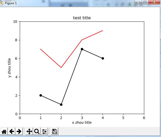
In [39]: plt.plot([1,2,3,4],[2,1,7,6], color=‘black‘, marker=‘o‘)
Out[39]: [<matplotlib.lines.Line2D at 0x17bb7f98>]

In [40]: plt.plot([1,2,3,4],[7,5,8,9], color=‘red‘)
Out[40]: [<matplotlib.lines.Line2D at 0x17c07940>]

In [41]: plt.title(‘test title‘)
Out[41]: Text(0.5, 1.0, ‘test title‘)

In [42]: plt.xlabel(‘x zhou title‘)
Out[42]: Text(0.5, 0, ‘x zhou title‘)

In [43]: plt.ylabel(‘y zhou title‘)
Out[43]: Text(0, 0.5, ‘y zhou title‘)

In [44]: plt.xlim(0,6)
Out[44]: (0, 6)

In [45]: plt.ylim(0,10)
Out[45]: (0, 10)

In [46]: plt.show()
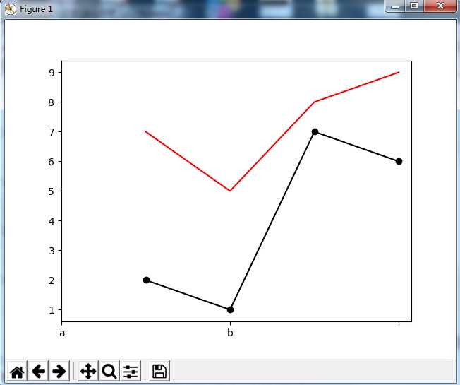
指定刻度名
In [47]: plt.plot([1,2,3,4],[2,1,7,6], color=‘black‘, marker=‘o‘)
Out[47]: [<matplotlib.lines.Line2D at 0x17befdd8>]

In [48]: plt.plot([1,2,3,4],[7,5,8,9], color=‘red‘)
Out[48]: [<matplotlib.lines.Line2D at 0x1a934710>]

In [50]: plt.xticks(np.arange(0,5,2), [‘a‘,‘b‘]) #刻度范围为一个可迭代的数据,规定刻度间距,其中第二个列表为指定刻度名称,在柱状图用常用
Out[50]:
([<matplotlib.axis.XTick at 0x1aa18438>,
  <matplotlib.axis.XTick at 0x1a9a5d30>,
  <matplotlib.axis.XTick at 0x1a9a5a58>],
 <a list of 2 Text xticklabel objects>)

In [51]: plt.show()
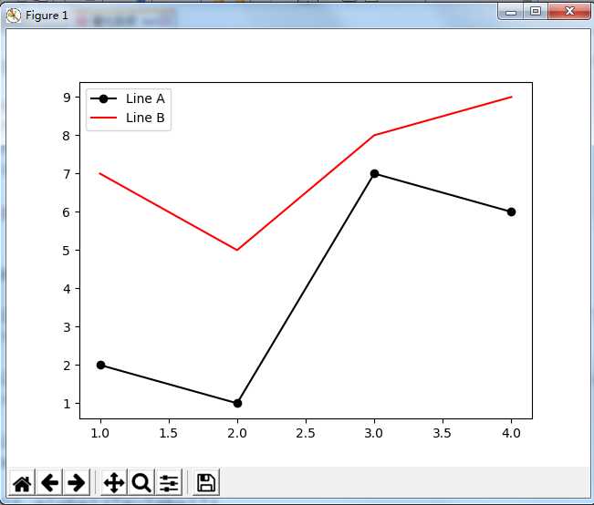
增加图例
In [52]: plt.plot([1,2,3,4],[2,1,7,6], color=‘black‘, marker=‘o‘,label=‘Line A‘)
Out[52]: [<matplotlib.lines.Line2D at 0x1aa49320>]

In [53]: plt.plot([1,2,3,4],[7,5,8,9], color=‘red‘, label=‘Line B‘)
Out[53]: [<matplotlib.lines.Line2D at 0x1ab10898>]

In [54]: plt.legend()
Out[54]: <matplotlib.legend.Legend at 0x1ab55400>

In [55]: plt.show()
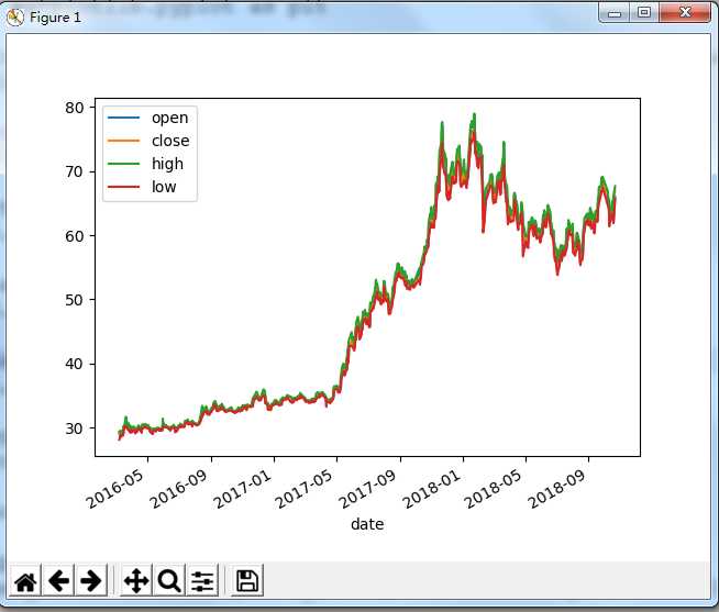
In [56]: df = pd.read_csv(‘111.csv‘, parse_dates=[‘date‘], index_col=‘date‘)[[‘open‘,‘close‘,‘high‘,‘low‘]]

In [57]: df.plot()
Out[57]: <matplotlib.axes._subplots.AxesSubplot at 0x1abf1860>

In [58]: plt.show()
上面的画的都是单图,如果想呈现多个图进行对比,那么就要用画布了,画布你就想象成一块黑板,然后把这块分割成多个区域,每个区域内都画个图,在这里叫子图
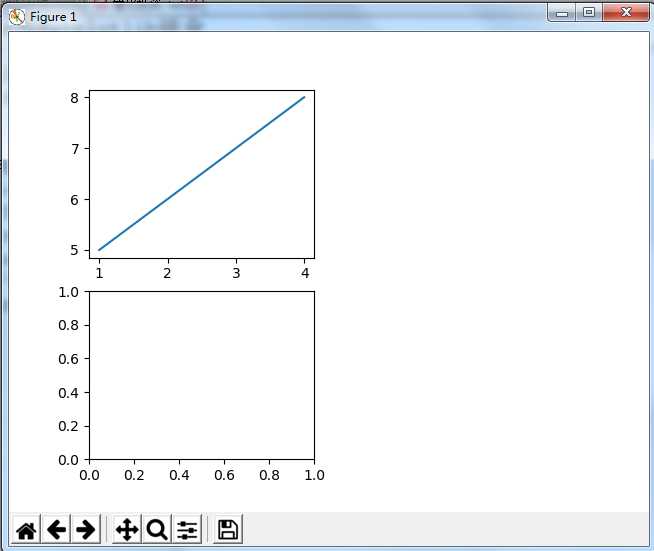
In [20]: fig = plt.figure()

In [21]: ax1 = fig.add_subplot(2,2,1)  #分成两行两列  占第一份

In [22]: ax1.plot([1,2,3,4],[5,6,7,8])  #给第一张图加数据
Out[22]: [<matplotlib.lines.Line2D at 0x32bdd10>]

In [23]: ax2 = fig.add_subplot(2,2,3)  #占第三份

In [24]: fig.show()
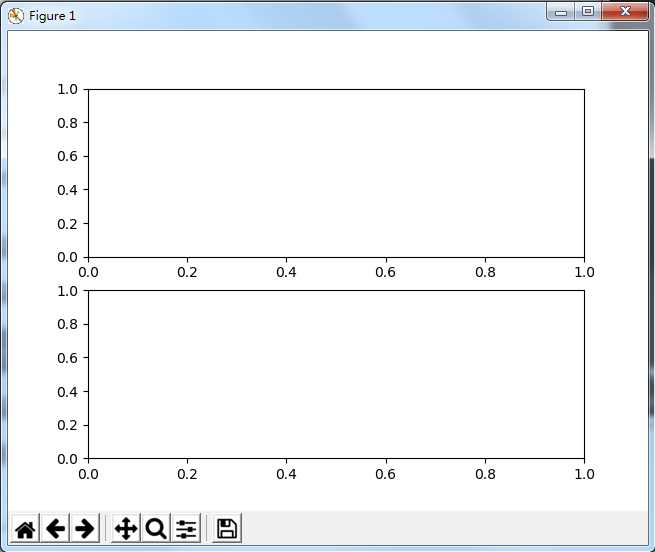
In [29]: fig = plt.figure()

In [30]: ax1 = fig.add_subplot(2,1,1)  #分成两行一列  占第一份

In [31]: ax2 = fig.add_subplot(2,1,2)  #占第二份

In [32]: fig.show()
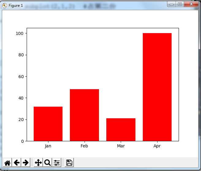
In [83]: data = [32, 48, 21, 100]

In [84]: labels = [‘Jan‘, ‘Feb‘, ‘Mar‘, ‘Apr‘]

In [85]: plt.bar(np.arange(len(data)), data, color=‘red‘)
Out[85]: <BarContainer object of 4 artists>

In [86]: plt.xticks(np.arange(len(data)), labels)
Out[86]:
([<matplotlib.axis.XTick at 0x1b97a390>,
  <matplotlib.axis.XTick at 0x1c4b3d68>,
  <matplotlib.axis.XTick at 0x1c4b3358>,
  <matplotlib.axis.XTick at 0x1c5062e8>],
 <a list of 4 Text xticklabel objects>)

In [87]: plt.show()
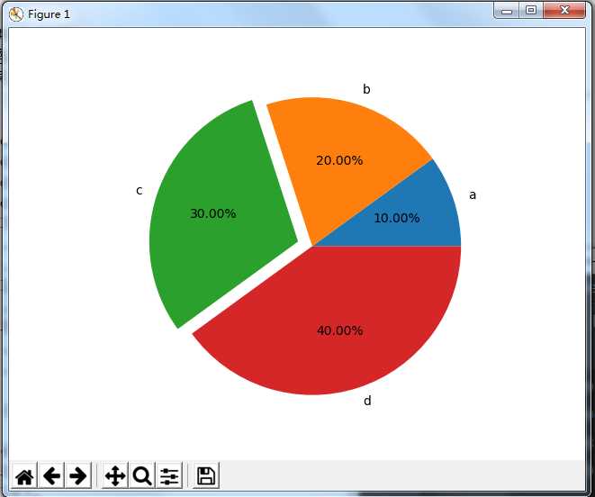
In [39]: plt.pie([10,20,30,40],labels=[‘a‘,‘b‘,‘c‘,‘d‘],autopct=‘%.2f%%‘,explode=[0,0,0.1,0])
Out[39]:
([<matplotlib.patches.Wedge at 0x109d2970>,
  <matplotlib.patches.Wedge at 0x109d2430>,
  <matplotlib.patches.Wedge at 0x109d21b0>,
  <matplotlib.patches.Wedge at 0x32a8b10>],
 [Text(1.04616,0.339919,‘a‘),
  Text(0.339919,1.04616,‘b‘),
  Text(-1.14127,0.37082,‘c‘),
  Text(0.339919,-1.04616,‘d‘)],
 [Text(0.570634,0.18541,‘10.00%‘),
  Text(0.18541,0.570634,‘20.00%‘),
  Text(-0.66574,0.216312,‘30.00%‘),
  Text(0.18541,-0.570634,‘40.00%‘)])

In [40]: plt.axis(‘equal‘)  #让饼图平铺  不是斜的
Out[40]:
(-1.2128537683838656,
 1.105374020036155,
 -1.1179348077041187,
 1.1179347975732619)

In [41]: plt.show()
matplotlib.finanace子包有许多绘制金融相关图的函数接口(如果matplotlib模块没有finance,可以下载这个mpl_finance)
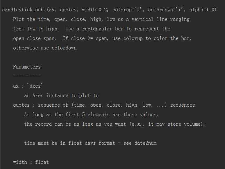
绘制k线图:matplotlib.finanace.candlestick_ochl函数
In [21]: import matplotlib.pyplot as plt
In [22]: import mpl_finance as fin
#用于把dataframe对象里的时间对象转换成python的时间对象
In [23]: from matplotlib.dates import date2num
In [24]: df = pd.read_csv(‘111.csv‘,parse_dates=[‘date‘], index_col=[‘date‘])[[‘open‘,‘close‘,‘high‘,‘low‘]]
In [25]: df
Out[25]:
open close high low
date
2016-03-08 29.022 29.321 29.368 28.094
2016-03-09 28.872 29.396 29.462 28.347
2016-03-10 29.022 28.797 29.312 28.759
2016-03-11 28.638 29.078 29.134 28.544
2016-03-14 29.031 29.143 29.574 28.947
2016-03-15 29.087 29.378 29.499 28.712
2016-03-16 29.134 30.099 30.221 29.087
2016-03-17 30.071 29.977 30.324 29.865
2016-03-18 30.277 30.090 30.371 29.865
2016-03-21 30.343 30.755 31.663 30.202
2016-03-22 30.586 30.071 30.951 29.977
2016-03-23 30.249 30.221 30.689 30.052
2016-03-24 30.043 29.790 30.061 29.743
2016-03-25 29.799 30.033 30.727 29.640
2016-03-28 30.071 29.471 30.305 29.368
2016-03-29 29.612 29.275 29.752 29.172
2016-03-30 29.602 29.968 30.033 29.527
2016-03-31 30.061 29.799 30.146 29.705
2016-04-01 29.818 29.902 29.940 29.237
2016-04-05 29.696 29.977 30.165 29.509
2016-04-06 29.771 29.734 29.940 29.640
2016-04-07 29.874 29.387 29.940 29.378
2016-04-08 29.228 29.190 29.293 29.078
2016-04-11 29.340 29.518 29.827 29.340
2016-04-12 29.499 29.556 29.743 29.415
2016-04-13 29.790 29.893 30.221 29.715
2016-04-14 30.052 29.996 30.333 29.865
2016-04-15 30.005 29.968 30.071 29.865
2016-04-18 29.790 29.780 30.061 29.518
2016-04-19 29.977 29.912 30.015 29.743
... ... ... ... ...
2018-09-03 61.980 62.109 62.376 61.495
2018-09-04 62.228 64.159 64.287 61.921
2018-09-05 63.772 62.178 64.000 62.178
2018-09-06 62.100 61.320 62.520 61.010
2018-09-07 61.880 62.780 63.500 61.600
2018-09-10 62.600 62.030 62.870 61.600
2018-09-11 62.000 61.680 62.580 61.250
2018-09-12 61.310 60.600 61.460 60.280
2018-09-13 61.780 62.400 62.400 61.010
2018-09-14 62.570 63.300 63.760 62.420
2018-09-17 62.300 62.510 63.180 62.250
2018-09-18 62.150 64.120 64.300 62.100
2018-09-19 64.090 65.150 65.800 63.810
2018-09-20 65.200 64.800 65.560 64.610
2018-09-21 65.280 67.490 67.500 64.970
2018-09-25 66.900 67.190 67.730 66.480
2018-09-26 67.230 67.960 69.000 66.830
2018-09-27 67.730 67.200 67.750 66.860
2018-09-28 67.500 68.500 69.100 67.440
2018-10-08 66.800 64.780 66.840 64.710
2018-10-09 64.630 65.000 65.380 64.330
2018-10-10 65.090 64.650 65.580 64.200
2018-10-11 62.100 61.850 63.200 61.380
2018-10-12 62.500 63.870 64.250 62.300
2018-10-15 63.900 63.200 64.440 63.090
2018-10-16 63.350 64.000 65.180 63.330
2018-10-17 65.170 64.160 65.320 62.410
2018-10-18 63.490 62.450 63.520 62.250
2018-10-19 61.990 65.620 66.100 61.880
2018-10-22 66.010 66.990 67.650 65.620
[641 rows x 4 columns]
#由于构筑蜡烛图的时候,第二参数必须要转入一个列表,列表第一个为是时间,而且必须要求为python里的时间戳对象
In [26]: df[‘time‘] = date2num(df.index.to_pydatetime()) #series对象不支持转成时间戳对象,而索引可以
In [27]: df
Out[27]:
open close high low time
date
2016-03-08 29.022 29.321 29.368 28.094 736031.0
2016-03-09 28.872 29.396 29.462 28.347 736032.0
2016-03-10 29.022 28.797 29.312 28.759 736033.0
2016-03-11 28.638 29.078 29.134 28.544 736034.0
2016-03-14 29.031 29.143 29.574 28.947 736037.0
2016-03-15 29.087 29.378 29.499 28.712 736038.0
2016-03-16 29.134 30.099 30.221 29.087 736039.0
2016-03-17 30.071 29.977 30.324 29.865 736040.0
2016-03-18 30.277 30.090 30.371 29.865 736041.0
2016-03-21 30.343 30.755 31.663 30.202 736044.0
2016-03-22 30.586 30.071 30.951 29.977 736045.0
2016-03-23 30.249 30.221 30.689 30.052 736046.0
2016-03-24 30.043 29.790 30.061 29.743 736047.0
2016-03-25 29.799 30.033 30.727 29.640 736048.0
2016-03-28 30.071 29.471 30.305 29.368 736051.0
2016-03-29 29.612 29.275 29.752 29.172 736052.0
2016-03-30 29.602 29.968 30.033 29.527 736053.0
2016-03-31 30.061 29.799 30.146 29.705 736054.0
2016-04-01 29.818 29.902 29.940 29.237 736055.0
2016-04-05 29.696 29.977 30.165 29.509 736059.0
2016-04-06 29.771 29.734 29.940 29.640 736060.0
2016-04-07 29.874 29.387 29.940 29.378 736061.0
2016-04-08 29.228 29.190 29.293 29.078 736062.0
2016-04-11 29.340 29.518 29.827 29.340 736065.0
2016-04-12 29.499 29.556 29.743 29.415 736066.0
2016-04-13 29.790 29.893 30.221 29.715 736067.0
2016-04-14 30.052 29.996 30.333 29.865 736068.0
2016-04-15 30.005 29.968 30.071 29.865 736069.0
2016-04-18 29.790 29.780 30.061 29.518 736072.0
2016-04-19 29.977 29.912 30.015 29.743 736073.0
... ... ... ... ... ...
2018-09-03 61.980 62.109 62.376 61.495 736940.0
2018-09-04 62.228 64.159 64.287 61.921 736941.0
2018-09-05 63.772 62.178 64.000 62.178 736942.0
2018-09-06 62.100 61.320 62.520 61.010 736943.0
2018-09-07 61.880 62.780 63.500 61.600 736944.0
2018-09-10 62.600 62.030 62.870 61.600 736947.0
2018-09-11 62.000 61.680 62.580 61.250 736948.0
2018-09-12 61.310 60.600 61.460 60.280 736949.0
2018-09-13 61.780 62.400 62.400 61.010 736950.0
2018-09-14 62.570 63.300 63.760 62.420 736951.0
2018-09-17 62.300 62.510 63.180 62.250 736954.0
2018-09-18 62.150 64.120 64.300 62.100 736955.0
2018-09-19 64.090 65.150 65.800 63.810 736956.0
2018-09-20 65.200 64.800 65.560 64.610 736957.0
2018-09-21 65.280 67.490 67.500 64.970 736958.0
2018-09-25 66.900 67.190 67.730 66.480 736962.0
2018-09-26 67.230 67.960 69.000 66.830 736963.0
2018-09-27 67.730 67.200 67.750 66.860 736964.0
2018-09-28 67.500 68.500 69.100 67.440 736965.0
2018-10-08 66.800 64.780 66.840 64.710 736975.0
2018-10-09 64.630 65.000 65.380 64.330 736976.0
2018-10-10 65.090 64.650 65.580 64.200 736977.0
2018-10-11 62.100 61.850 63.200 61.380 736978.0
2018-10-12 62.500 63.870 64.250 62.300 736979.0
2018-10-15 63.900 63.200 64.440 63.090 736982.0
2018-10-16 63.350 64.000 65.180 63.330 736983.0
2018-10-17 65.170 64.160 65.320 62.410 736984.0
2018-10-18 63.490 62.450 63.520 62.250 736985.0
2018-10-19 61.990 65.620 66.100 61.880 736986.0
2018-10-22 66.010 66.990 67.650 65.620 736989.0
[641 rows x 5 columns]
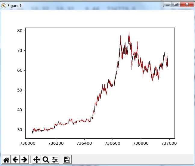
In [28]: fig = plt.figure()
In [29]: ax = fig.add_subplot(1,1,1) #创建子图实例,传入第一参数
In [30]: arr = df[[‘time‘,‘open‘,‘close‘,‘high‘,‘low‘]].values #获取序列化值,传入第二参数
In [31]: fin.candlestick_ochl(ax,arr) #把子图和数据传入
In [33]: fig.show()
一个自动获取财经数据的模块,需要下载pandas requests beautifulsoup4模块才能使用
获取到数据就是df对象
使用指南 http://tushare.org/
pip install tushare
In [1]: import tushare as ts

In [2]: ts.get_k_data(‘601318‘)
Out[2]:
           date    open   close    high     low     volume    code
0    2015-08-07  31.956  32.483  32.819  31.774  1524162.0  601318
1    2015-08-10  32.589  33.634  33.969  32.177  2198393.0  601318
2    2015-08-11  33.451  33.423  34.209  33.260  1664871.0  601318
3    2015-08-12  33.068  32.388  33.317  32.368  1333463.0  601318
4    2015-08-13  32.311  32.656  32.857  32.110  1100029.0  601318
5    2015-08-14  32.761  32.483  32.838  32.397  1155956.0  601318
6    2015-08-17  32.023  31.602  32.100  31.247  1521704.0  601318
7    2015-08-18  31.659  29.991  32.234  29.943  2103894.0  601318
8    2015-08-19  29.665  30.106  30.327  29.234  1614533.0  601318
9    2015-08-20  29.713  29.282  30.097  29.253  1098640.0  601318
10   2015-08-21  29.196  28.170  29.857  28.084  2058581.0  601318
11   2015-08-24  27.308  25.352  27.317  25.352  4032962.0  601318
12   2015-08-25  24.250  24.068  26.407  23.627  4316161.0  601318
13   2015-08-26  24.154  25.266  26.167  24.077  3826691.0  601318
14   2015-08-27  26.263  27.796  27.796  25.851  3939984.0  601318
15   2015-08-28  28.276  28.419  29.129  27.595  3319339.0  601318
16   2015-08-31  27.662  29.033  29.090  27.336  2894666.0  601318
17   2015-09-01  28.304  28.908  28.927  27.461  3690911.0  601318
18   2015-09-02  27.940  28.736  28.985  27.825  3735058.0  601318
19   2015-09-07  28.419  27.681  29.023  27.413  1363133.0  601318
20   2015-09-08  27.662  28.525  28.630  27.662  1255286.0  601318
21   2015-09-09  28.793  29.141  29.565  28.552  1430501.0  601318
22   2015-09-10  29.006  29.189  29.276  28.745   878888.0  601318
23   2015-09-11  29.083  28.774  29.382  28.552   708262.0  601318
24   2015-09-14  28.900  29.063  29.121  27.704  2206746.0  601318
25   2015-09-15  28.543  28.408  28.726  27.964  1183297.0  601318
26   2015-09-16  28.282  29.459  30.057  28.032  1148146.0  601318
27   2015-09-17  29.401  29.179  30.066  29.025  1016069.0  601318
28   2015-09-18  29.333  29.478  29.989  29.276   856438.0  601318
29   2015-09-21  29.131  29.854  30.037  28.977   810319.0  601318
..          ...     ...     ...     ...     ...        ...     ...
610  2018-02-05  74.400  75.710  75.950  74.300   948054.0  601318
611  2018-02-06  73.850  73.770  74.700  72.500  2049666.0  601318
612  2018-02-07  74.600  71.380  74.650  70.500  1747840.0  601318
613  2018-02-08  70.610  68.990  71.500  68.370  1530108.0  601318
614  2018-02-09  66.500  64.430  66.970  62.200  2492029.0  601318
615  2018-02-12  64.660  64.960  65.650  64.000  1029611.0  601318
616  2018-02-13  66.200  67.020  68.350  66.060  1147957.0  601318
617  2018-02-14  67.500  68.890  69.190  67.200   646501.0  601318
618  2018-02-22  70.230  69.770  70.420  69.230   783649.0  601318
619  2018-02-23  70.250  70.640  71.460  69.830   556011.0  601318
620  2018-02-26  70.990  70.800  71.580  69.600   693840.0  601318
621  2018-02-27  71.020  69.810  71.190  69.470   780994.0  601318
622  2018-02-28  69.200  67.760  69.240  67.700   782170.0  601318
623  2018-03-01  67.180  68.930  69.380  66.880   663296.0  601318
624  2018-03-02  68.000  67.680  68.660  67.450   581439.0  601318
625  2018-03-05  67.660  67.880  68.590  67.000   609823.0  601318
626  2018-03-06  68.400  69.320  69.390  67.400   657077.0  601318
627  2018-03-07  68.980  68.780  70.180  68.180   590555.0  601318
628  2018-03-08  69.060  70.540  70.840  68.760   692681.0  601318
629  2018-03-09  71.000  70.890  71.460  70.310   476222.0  601318
630  2018-03-12  71.600  71.120  71.860  70.600   583351.0  601318
631  2018-03-13  71.200  69.420  71.350  69.180   609492.0  601318
632  2018-03-14  68.850  68.820  69.200  68.260   514760.0  601318
633  2018-03-15  68.410  70.490  70.700  68.400   627110.0  601318
634  2018-03-16  70.700  70.510  71.950  70.450   701326.0  601318
635  2018-03-19  70.890  73.810  73.880  70.480   924499.0  601318
636  2018-03-20  73.100  74.090  74.190  72.700   659778.0  601318
637  2018-03-21  76.700  73.820  76.710  73.030  1367485.0  601318
638  2018-03-22  73.510  72.880  74.170  71.680   902877.0  601318
639  2018-03-23  70.000  70.300  70.770  69.420  1486954.0  601318

[640 rows x 7 columns]
标签:pip range otl 需要 5.0 时间 自动 from time
原文地址:https://www.cnblogs.com/xinsiwei18/p/9817983.html