标签:hold after softmax plot home row intersect eth pil
Using Open-Source Implementation
We have learned a lot of NNs and ConvNets architectures
It turns out that a lot of these NN are difficult to replicated. because there are some detail that may not presented on its paper. There are some other reasons like:
Learning decay
Parameter tuning
A lot of deep learning researchers are opening sourcing thir code into Internet on sites like Github.
If you see a research paper and you want to build over it, the first thing you should do is to look for an open source implementation for this paper.
Some advantage of doing this is that you might download the network implementation along with its parameters/weights. The author might used a multiple GPUs and some weeks to reach this result and its right in front of you after you download it.
Transfer learning
If you are using a specific Nn architecture that has been trained before, you can use this pretrained parameters/weights instead of random initialization to solve your problem.
It can help you boost the performance of the NN.
The pretrained models might have trained a large datasets like ImageNet, Ms COCO, or pascal and took a lot of time to learn those parametters/weights withh optimized hyperparameters. This can save you a lot of time.
Lets see an example:
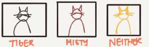
Lets say you have a cat classification problem which contains 3 classes Tigger, Misty and
neither.
You don‘t have much a lot of data to train a NN on these images
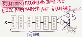
Andrew recommends to go online and download a good NN with its weights, remove
the softmax activation layer and put your own one and make the network learn only the new layer while other layer weights are fixed/frozen
Frameworks have options to make the parameters frozen in some layers using t
trainable=0 or freeze=0
One of the tricks that can speed up your training, is to run the pretrained NN without
final softmax layer and get an intermediate representation of your images and save them disk. And then use these representation to a shallow NN network. This can save you the
time needed to run an image through all the layers.
Its like converting your images into vectors.
Another example:
What if in the last example you have a lot of pictures for your cats.
One thing you can do is to freeze few layers from the beginning of the pretrained
network and learn the other weights in the network
Some other idea is to through away the layers that aren‘t freeze and put your own layers
there.
Another example:
If you have enough data, you can fine tune all the layers in your pretrained network but
but don‘t random initialize the parameters, leave the learned parameters as it is and learn
from there.
Data Augmentation
If data is increase, your deep NN will perform better. Data augmentation is one of the techniques that deep learning uses to increase the performance of deep NN.
The majority of computer vision applications needs more data right now.
Some data augmentation methods that are used for computer vision tasks includes:
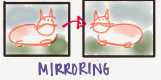
Mirroring
Random cropping
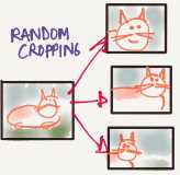
The issue with this technique is that you might take a wrong crop.
The solution is to make your crops big enough.
Rotation.
Shearing
Local warping
Color shifting
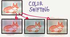
For example, we add to R,G and B some distortions that will make the image
identified as the same for the human but is different for the computer.
In practice the added value are pulled from some probability distribution and these
shits are some small.
Makes your algorithm more robust in changing color in images.
There are an algorithm which is called PCA color augmentation that decides the
shits are some small
Implementing distortions during trainging:
You can use a different CPU thread to make you a distorted mini batchs while you
are training your NN.
Data Augmentation has also some hyperparameters. A good place to start is to find an
openf source data augmentation implementation and then use it to fine tune these
hyperparameters.
state of Computer Vision
For a specific problem we may have a little data for it or a lots of data.
Speech recognition problems for example has a big amount of data, while image recognition has a medium amount of data and the object detection has a small amount ofdata nowadays.
If you problem has a large amount of data, researchers are tend to use:
Simpler algorithms
Less hand engineering
If you don‘t have that much data people are tend to try more hand engineering for the problem "Hacks". Like choosing a more complex NN architecture.
Because we haven‘t that much data in a lot of computer vision problems, It relies a lot on hand engineering.
We will see in the next chapter that because the object detection has a less data, a more complex NN architectures will be presented.
Tips for doing well on benchmarks/winning competitions:
Ensembling.
Train several networks independently and average their outputs. Merging down
some classifiers.
After you decide the best architecture for your problem, initialize some fo that some
of that randomly and train them independently
This can give you a push by 2%
But this will slow down your production by the number of the ensembles. Also it
takes more memory as it saves all the models in the memory.
People use this in competitions but few uses this in a real production
Multi-crop at test time.
Run classifier on multiple versions of test versions and average results.
There is a technique called 10 crops that uses this.
This can give you a better result in the production.
Use open source code
Use architectures of networks published in the literature
Use open source implementations if possible.
Use pretrained models and fine-tune on your dataset.
Object detection
Learn how to apply your knowledge of CNNs to one of the thoughest but hottest field of computer vision: Object detection.
Object Localization
Object detection is one from the areas that deep learning is doing great in the past two years.
What are localization and detection?
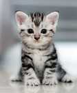
Image Classfication:
Classify an image to a specific class. The whole image represents one class. We don‘t
want to know exactly where are the object. Usually only one object is presented.
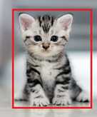
Classification with localization:
Given an image we want to learn the class of the image and where are the class
location in the image. We need to detect a class and a rectangle of where that object
is. Usually only one object is presented.
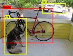
Object detection:
Given an image we want to detect all the object in the image that belong to a specific
classes and give their location. An image can contain more than one object with
different classes.
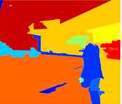
Semantic Segmentation:
We want to Label each pixel in the image with a category label. Semantic
Segmentation Don‘t differentiate instances, only care about pixels. It detects no
objects just pixels.
If there are two objects of the same class is intersected, we won‘t be able to separate
them.
Instance Segmentation
This is like the full problem. Rather than we want to predict the bounding box, we
want to know which pixel label but also distinguish them.
To make image classification we use a Conv Net with a softmax attached to the end of it.
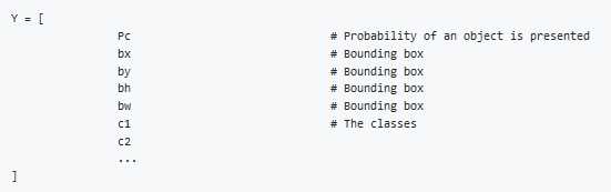
To make classification with localization we use a Conv Net with a softmax attached to the end of it and a four number bx,by,bh and bw to tell you the location of the class in the image.
The dataset should contain this four numbers with the class too.
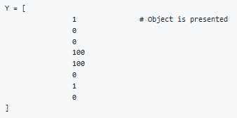
Defining the target label Y in classification with localization problem:
Example(Object is presented):
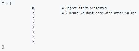
Example(When object isn‘t presented):
The loss function for the Y we have created (Example of the square error):
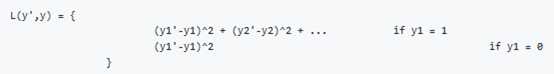
In practice we use logistic regression for pc, log likely hood loss for classes, and squared
error for the bounding box.
Landmark Detection
In some of the computer vision problems you will need to output some points. That is called landmark detection.
For example, if you are working in a face recognition problem you might want some points on the face like corners of the eyes, corners of the mouth, and corners of the nose and so on. This can help in a lot of application like detecting the pose of the face.
Y shape for the face recognition problem that needs to output 64 landmarks:
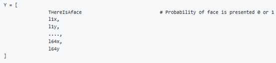
Another application is when you need to get the skeleton of the person using different landmarks/points in the person which helps in some application.
Hint, in your labeled data, if l1x,l1y is the left corner of left eye, all other l1x,l1y of the other examples has to be the same.
Object Detection
We will use a Conv net to solve the object detection problem using a technique called the sliding windows detection algorithm.
For example lets say we are working on Car object detection
The first thing, we will a Conv net on a cropped car objects and non car images
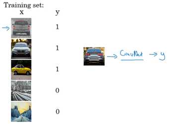
After we finish training of this Conv net we will then use it with the sliding windows technique
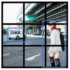
Sliding windows detection algorithm:
Decide a rectangle size.
Split your image into rectangles of the size you picked. Each region should be covered.
You can use some strides.
For each rectangle feed the image into the Conv net and decide if it‘s a car or not.
Pick larger/smaller rectangles and repeat the process from 2 to 3
Store the rectangles that contains the cars.
If two or more rectangles intersects choose the rectangle with best accuracy.
Disadvantage of sliding window is the computation time.
In the era of machine learning before deep learning, people ussed a hand crafted linear classifiers that classifiers the object and then use the sliding window technique. The linear classier make it a cheap computation. But in the deep learning era that is so computational expensive due to the complexity of the deep learning model.
To solve this problem, we can implement the sliding windows with a Convolutional approach.
One other idea is to compress your deep learning model.
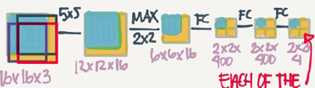
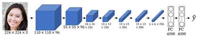
Convolutional Implementation of Sliding Windows
Truning FC layer into convolutional layer(predict image class from four classes):
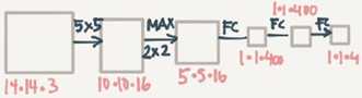
As you can see in the above image, we turned the FC layer into a Conv layer using a
convolution with the width and height of the filter is the same as the with and height of
the input.
Convolution implementation of sliding windows
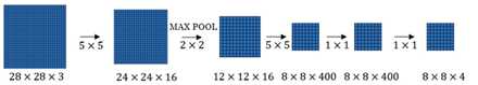
First lets consider that the Conv net you trained in like this (No FC all is conv layer):
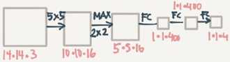
Say now we have a 16*16*3 image that we need to apply the sliding windows in. By the normal implementation that have been mentioned in the section before this, we could run this Conv net four thimes each rectangle size will be 16*16
The convolution implementation will be as follows:
Simply we have feed the image into the same Conv Net we have trained.
The left cell of the result "The blue one" will represent the first sliding window of the normal implementation.The Other cells will represent the others.
Its more efficient because it now shares the computations of the four times needed.
Another example would be:
This example has a total of 16 sliding windows that shares the computation togethter.
The weakness of the algorithm is that the position of the rectangle wont be so accurate. Maybe none of the rectangles is exactly on the object you want to recognize.
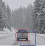
In the red rectangle we want in blue the best car rectangle.
Bounding Box Predictions
A better algorithm than the onedescribed in the last section is the YOLO algorithm
YOLO stands for you only look once and was developed back in 2015.
Yolo Algorithm:
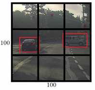
Lets say we have an image of 100*100
Place a 3*3 grid on the image. For more smother results you should use 19*19 for the
100*100
Appy the classification and localization algorithm we discussed in a previsous section to
each section of the grid. bx and by will represent the center point of the object in each
grid and will be relative to the box so the range is between 0 and 1 while bh and bw will
represent the height and width of the object which can ge greater than 0.0 but still float
point.
Do everything at once with the convolution sliding window. If Y shape is 1*8 as we
discussed before then the output of the 100*100 image should be 3*3*8 which
corresponds to 9 cell results.
Merging the results using predicted localization mid point.
We have a problem if we have found more than one object in one grid box.
One of the best advantages that makes the YOLO algorithm popular is that it has a great speed and a Conv net implementation.
How is YOLO different from other Object detectors? YOLO uses a single CNN network for both classification and localizing the object using bounding boxes.
Intersection Over Union
Intersection Over Union is a function used to evaluate the object detection algorithm
It computes size of intersection and divide it by the union. More generally LOU is a measure of the overlap between two bounding boxes.
For example:
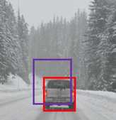
The red is the labeled output and the purple is the predicted output.
To computeIntersection Over Union we first compute the union are of the two rectangles
which is "the first rectangle+second rectangle" Then compute the intersection are
between these two rectangle.
Finally IOU=intersection area/Union area
If IOU>=0,5 then its good. Th best answer will be 1.
The hight the IOU the better is the accuracy.
Non-max Suppression
One of the problems we have addressed in YOLO is that it can detect an object multiple times.
Non-max Suppression is a way make sure that YOLO detects the object just once.
For example
Each car has two or more detections with different probabilities. This came from some of the grids that thinks that this is the center point of the object.
Non-max suppression algorithm
Lets assume that we are targeting one class as an output
Y shape should be [Pc,bx,by,bh,bw] Where Pc is the probability if that object occurs
Discard all boxes with Pc<0.6
While there are any remaining boxes:
Pick the box with the largest Pc Output that as a prediction
Discard any remaining box with IOU<0.5 with the box output in the previous step.
If there are multiple classes/object types c you want to detect, you should run the Non-max suppression c times.
Anchor Boxes
In YOLO, a grid only detects one object. What if a grid cell want to detect multiple object?
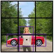
Car and person grid is same here.
In practice this happens rarely.
The ideal of Anchor boxes help us solving this issue.
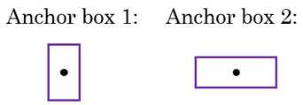
If Y=[Pc,bx,by,bh,bw,c1,c2,c3] Then to use two anchor boxes like this:
Y=[Pc,bx,by,bh,bw,c1,c2,c3,Pc,bx,by,bh,bw,c1,c2,c3] we simply have repeated the one
anchor Y
The two anchor boxes you choose should be know as a shape:
So previously, each object in training image is assigned to grid cell that contains that object‘s midpoint.
With two anchor boxes,Each object in training image is assigned to grid cell that contains object‘s midpoint and anchor box for the grid cell with highest IoU. You have to check where your object should be based on its rectangle closest to which anchor box.
Example of data:
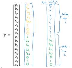
Where the car was near the anchor 2 than anchor 1
You may have two or more anchor boxes but you should know their shapes
How do you choose the anchor boxes and people used to just choose them by hand
you know choose a maybe five or ten anchor ball shapes that spans a variety of shapes
that see to cover the types of objects you seem to detect as a much
Anchor boxes allows you algorithm to specialize, means in our case to easily detect wider images or taller ones.
YOLO Algorithm
YOLO is a state-of-the-art object detection model that is fast and accurate
Lets sum up and introduction the whole YOLO algorithm given an example
Suppose we need to do object detection for our autonomous driver system. It needs to identify three classes:
Pedestrain(Walks on ground)
Car
Motorcycle
We decide to choose two anchor boxes, a taller and a wide one
Like we said in practice they use five or more anchor boxes hand made or generated
using k-means
Our labeled Y shape will be [Ny, HeightOf Grid, WidthOfGrid,16] each row is as follow:
[Pc,bx,by,bh,bw,c1,c2,c3,Pc,bx,by,bh,bw,c1,c2,c3]
Your dataset could be an image with a multiple labels and rectangle for each label, we should go to your dataset and make the shape and values of Y like we agreed.
An example:
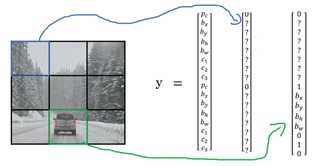
We first initialize all of them to zeros and ?, then for each label and rectangle choose its
closest grid point then the shape to fill it and then the best anchor point based on the
IOU. So that the shape of Y for one image should be [HeightOfGrid,WidthOfGrid,16]
Train the labeled images on a Conv net. you should receive an output of [HeightOfGrid,WidthOfGrid,16] for our case.
To make predictions, run the Conv net. You should receive an output of [HeightOfGrid,WidthOfGrid,16] for our case.
To make predictions, run the Conv net on an image and run Non-max suppression algorithm for each class you have in our case there are 3 classes.
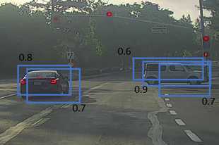
You could get something like that:
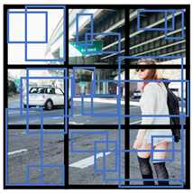
Total number of generated boxes are grid_width*grid_height*no_of_anchors=3*3*2
By removing the low probability predictions you should have:
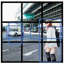
Then get the best probability followed by the IOU filtering, For each class(pedestrian
,car,motorcycle) use non-max suppression to generate final predictios.
YOLO are not good at detecting smaller object.
Region Proposals(R-CNN)
R-CNN is an algorithm that also makes an object detection
YOLO tells that its faster:
Our model has several advantages over classifier-based system. It looks at the whole
image at test time so its predictions are informed by global context in the image. It also
makes preditions with a single network evaluation unlike systems like R-CNN which
require thousands for single image. This makes it extremely fast, more than 1000x faster
than R-CNN and 100x faster then Fast R-CNN. See our paper for more details on the full
system.
But one of the downsides of YOLO that it process a lot of areas where no objects are present.
R-CNN stands for regions with Conv Nets.
R-CNN tries to pick a few windows and run a Conv net(your confident classifier) on top of them.
The algorithm R-CNN uses to pick windows is called a segmentation algorithm. Outputs something like this:
If for example the segmentation algorithm produces 2000 blob then we should run our classifier/CNN on top of these blobs.
Most of the implementation of faster R-CNN are still slower than YOLO.
Andew NG thinks that the idea behind YOLO is better than R-CNN because you are able to do all the thing in just one time instead of two times.
What is face recognition?
Face recognition system identifies a persons face. It can work on both images or videos.
Liveness detection within a video face recognition system prevents the network from identifiying a real picture in an image. It can be learned by supervised deep learning using a dataset for live human and in-live human and sequence lerning.
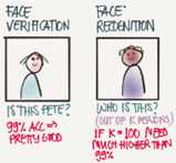
Face verificaton vs. face recognition:
Verification:
Input image,name/ID(1:1)
Output whether the input image is that of the claimed person.
"is this the claimed person?"
Recognition:
Has a database of k persons
Get an input image
Output ID if the image is any of the k persons(or not recognized)
"who is this person?"
We can use a face verification system to make a face recofnition system. The accuracy of the verification system has to high (around 99.9% or more) to be use accurately within a recognition system because the recognition system accuracy will be less than the verification system given a k persons.
One Shot Learning
One of the face recognition challenges is to solve a one shot problem
One shot Learning: A recognition system is able to recognize a person learning from a image
Historically deep learning doesn‘t work well with a small number of data
Instead to make this work, we will learn a similarity function:
d(img1,img2)=degree of difference between images.
We want d result to be low in case of the sace faces.
We use tau T as a threshold for d:
if d(img1,img2)<=T then the faces are the same.
Similarity function helps us solving the one shot learning. Also its robust to new inputs.
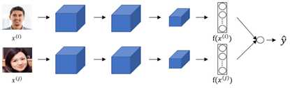
Siamese Network
We will implement the similarity function using a type of NNs called Siamease Network in which we can pass multiple inputs to the two or more networks with the same architecture parameters.
Siamese network architecture are as the following:
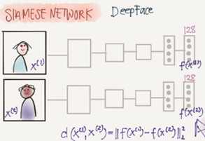
We make 2 identical conv nets which encodes an input image into a vector. In the above
vector shape is (128,)
The loss function will be d(x1,x2)=||f(x1)-f(x2)||2
If x1,x2 are the same person, we want d to be low. If they are different persons, we want
d to be high.
Triplet Loss
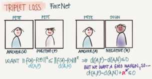
Triplet Loss is one of the loss functions we can use to solve the similarity distance in a Siamese network.
Our learning objective in the triplet loss function is to get the distance between an Anchor image and a positive or a negative image
Positive means same person, while negative means different person.
The triplet name came from that we are comapring an anchor A with a positive p and a negative N image.
Formally we want:
Positive distance to be less than negative distance
||f(A)-f(P)||2<=||f(A)-f(N)||2
Then
||f(A)-f(P)||2-||f(A)-f(N)||2<=0
To make sure the NN won‘t get an output of zeros easily:
||f(A)-f(P)||2-||f(A)-f(N)||2<=-alpha
Alpha is a small number. Sometimes its called the margin
Then
||f(A)-f(P)||2-||f(A)-f(N)||2+alpha<=0
Final Loss function:
Given 3 images(A,P,N)
L(A,P,N)=max(||f(A)-f(P)||2-||f(A)-f(N)||2+alpha,0)
J=Sum(A[i],P[i],N[i]),i) fo rall triplets of images.
You need multiple images of the same person in your dataset. Then get some triplets out of your dataset. Dataset should be big enough.
Choosing the triplets A,P,N:
During training if A,P,N are chosen randomly(Subjet to A and P are the same and A and
N aren‘t the same)
then one of the problems this constrain is easily satisfied
d(A,P)+alpha<=d(A,N)
So the NN wont learn much
What we want to do is choose triplets that are hard to train on
So for all the triplets we want this to be satisfied:
d(A,P)+alpha<=d(A,N)
This can be achieved by for example same poses!
Find more at the paper.
Commercial recognition systems are trained on a large datasets like 10/100 million image.
There are a lot of pretrained models and parameters online for face recognition.
Face Verification and Binary Classification
Triplet loss is one way to learn the parameters of a conv net for face recognition there‘s another way to learn these parameters as a straight binary classificaiton problem.
Learning the similarity funciton another way:
Learning the similarity function another way:
The final layer is sigmoid layer.
Y‘=wi*Sigmoid(f(x(i))-f(x(j)))+b where the subtraction is the Manhattan distance between
f(x(i)) and f(x(j))
Some other similarites can be Euclidean and Ki square similarity.
The NN here is Siamese means the top and bottom convs has the same parameters.
A good performance/deployment trick:
Pre-compute all the images that you are using as a comparison to the vector f(x(j))
When a new image that needs to be compared, get its vector f(x(i)) then put it with all
the pre computed vectors and pass it to the sigmoid function.
This version works quite as well as the triplet loss function.
Available implementations for face recognition using deep learning includes:
Openface
FaceNet
DeepFace
What is nerural style transfer?
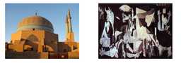
Neural style transfer is one of the application of Conv nets.
Nerural style transfer takes a content image c and a style image s and generated the content image G with the style of style image.
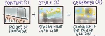
In order to implement this you need to look at the features extracted by the Conv net at the shallower and deeper layers
It uses a previously trained convolutional network like VGG, and builds on top of that. The idea of using a network trained on a different task and applying it to a new task is called transfer learning.
What are deep ConvNets learning
Visualizing what a deep network is learning
Given this AlexNet like Conv net
Pick a unit in a layer I, Find the nine image patches that maximize the unit‘s activation
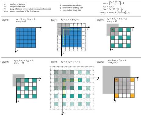
Notice that a hidden unit in layer one will see relatively small protion of NN,So fi you
plotted it it will match a small image I the shallower layers while it will get larger
image in deeper layers.
Repeat for other units and layers
It turns out that layer 1 are leanring the low level representations like color and edges.
You will find out that each layer are learning more complex representations.
The first layer was created using the weight of the first layers. Other images are generated using the receptive filed in the image that triggered the neuron to be max.
A good explanation on how to get receptive field givena layer:
Cost Function
We will define a cost function for the generated image that measures how good it is.
Given a content image C, a style image S, and a generated imageG:
J(G)=alpha*J(C,G)+betaJ(S,G)
J(C,G) measures how similar is the generated image to the Content image
J(S,G) measures how similar is the generated image to the Style image.
alpha and beta are relative weighting to the similarity and these are hyperparameters.
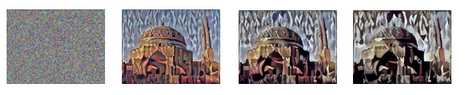
Find the generated image G:
Initiate G randomly
For example G:100*100*3
Use gradient descent to minimize J(G)
G=G-dG We compute the gradient iamge and use gradient decent to minimize the
cost function.
The iterations might be as following imiage:
To generate this:
You will go through this:
Content Cost Function
In the previous section we showed that we need a cost function for the content image and the style image to measure how similar is them to each other.
Say you use hidden layer l to compute content cost
If we choose l to be small(like layer 1). we will force the network to get similar output to
the original content image.
In practice l is not to shallow and not to deep but in the middle.
Use pre-trained ConvNet(E.g. VGG network)
Let a(c)[l] and a(G)[l] be the activation of layer l on the images.
If a(c)[l] and a(G)[l] are similar then they will have the same content
J(C,G) at a layer l=1/2||a(c)[l]-a(c)[G]||2
Style Cost Function
Meaning of the style of an image:
Say you are using layer l‘s activation to measure style
Define style as correlation between activations across channels
That means given an activation like this:
How correlate is the orange channel with the yellow channel?
Correlated means if a value appeared in a specific channel a specific value will
appear too(Depends on each other)
Uncorrelated means if a value appeared in a specific channel doesn‘t mean that
another value will appear(Not depend on each other)
The correlation of style image channels should appear in the generated image channels
The correlation of style image channels should appear in the generated image channels.
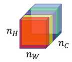
Style matrix(Gram matrix):
Let a(l)[i,j,k] be the activation at l with (i=H,j=W,k=C)
Also G(l)(S) is matrix of shape nc(l)*nc(l)
We call this matrix style matrix or Gram matrix
In this matrix each cell will tell us how correlated is a channel to another chanel
To populate the matrix we use these equations to compute style matrix of the style image
and the generated image.
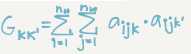
As it appears it‘s the sum of the multiplication of each member in the matrix.
To compute gram matrix efficiently:
Reshape activation from H X W X C to HW X C
Name the reshaped activation F.
G[l]=F*F.T
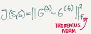
Finally the cost function will be as following
J(S,G) at layer l=(1/(2*H*W*C)^2)||G(l)(S)-G(l)(G)||2
And if you have used it from some layers
J(S,G)=Sum(lamda[l]*J(S,G)[l], for all layers)
Steps to be made if you want to create a tensorflow model for neural style transfer:
Create an Interactive Session
Load the content image.
Load the style image
Randomly initialize the image to be generated
Load the VGG 16 model
Build the Tensorflow graph:
Run the content image through the VGG16 model and compute the content cost
Run the style image through the VGG16 model and compute the style cost
Compute the total cost
Initialize the TensorFlow graph and run it for a large number of iterations, updating the
generated image at every step.
So far we have used the Conv nets for images which are 2D
Conv nets can work with 1D and 3D data as well
An example of 1D convolution
Input shape(14,1)
Applying 16 filters with F=5,S=1
Output shape will be 10*16
Applying 32 filters with F=5,S=1
Output shape will be 6*32
The general equation (N-F)/s+1 can be applied here but here it gives a vector rather than a 2D matrix.
1D data coms from a lot of resources such as waves, sounds,heartbeat signals.
In most of the applications that uses 1D data we use Recurrent Neural Network RNN.
3D data also are available in some application like CT scan:
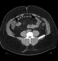
Example of 3D convolution:
Input shape(14,14,14,1)
Applying 16 filters with F=5,S=1
Output shape(10,10,10,16)
Applying 32 filters with F=5,S=1
Output shape will be (6,6,6,32)
Extras
Keras
Keras is a high-level neural networks API (programming framework), written in python and capable of running on top of several lower-level framworks including TensorFlow, Theano, and CNTK.
Keras was developed to enable deep learning engineers to build and experiment with different models vey quickly.
Just as TensorFlow is a high-level framework than Python, Keras is an even higher-level framework and provides additional abstractions.
Keras will work fine for many common models.
Layers in Keras:
Dense(Fully connected layers)
A linear function followed by a non linear function
Convolutional layer
Pooling layer.
Normalisation layer.
A batch normalization layer.
Flatten layer
Flatten a matrix into vector.
Activation layer
Different activations include: relu, tanh, sigmoid, and softmax
To train and test a model in Keras there are four steps
Create the model
Compile the model by calling model.compile(optimizer="…",loss="…",metrics=[accuracy])
Train the model on train data by calling model.filt(x=…,y=…,epochs=…,batch_size=…)
You can add a validation set while training too.
Test the model on test data by calling model.evaluate(x=…,y=…)
Summarize of step in Keras: Create->Compile->Fit/Train->Ealuate/Test
Model.summary() gives a lot of useful informations regarding your model including each layers inputs, outputs, and number of parameters at each layer.
To choose the Keras backend you should go to $HOME/.keras/keras.json and change the file to the desired backend like Theano or Tensorflow or whatever backend you want.
After you create the model you can run it in a tensorflow session without compling training, and testing capabilities.
You can save your model with model_save and load your model using model_load this will save your whole trained model to disk with the trained weights.
标签:hold after softmax plot home row intersect eth pil
原文地址:https://www.cnblogs.com/kexinxin/p/9904376.html