标签:one 控制 when scalar oar 下载 instead between var
优点:tf官方推荐格式,兼容大部分格式,采用二进制保存文件,在tf中处理效率最高
cs20的一个good example:
写tfrecord的pipeline
# Step 1: create a writer to write tfrecord to that file
writer = tf.python_io.TFRecordWriter(out_file)

# Step 2: get serialized shape and values of the image
shape, binary_image = get_image_binary(image_file)

# Step 3: create a tf.train.Features object
features = tf.train.Features(feature={'label': _int64_feature(label),
                                    'shape': _bytes_feature(shape),
                                    'image': _bytes_feature(binary_image)})

# Step 4: create a sample containing of features defined above
sample = tf.train.Example(features=features)

# Step 5: write the sample to the tfrecord file
writer.write(sample.SerializeToString())
writer.close()
读tfrecord的pipeline
# _parse_function可以定制,以适应各种类型

dataset = tf.data.TFRecordDataset(tfrecord_files)
dataset = dataset.map(_parse_function)

def _parse_function(tfrecord_serialized):
    features={'label': tf.FixedLenFeature([], tf.int64),
              'shape': tf.FixedLenFeature([], tf.string),
              'image': tf.FixedLenFeature([], tf.string)}

    parsed_features = tf.parse_single_example(tfrecord_serialized, features)

    return parsed_features['label'], parsed_features['shape'], parsed_features['image']
一个示例:
# 其中 使用queue部分 现在被tf.data代替,所以这部分应该用tf.data重写下
def _int64_feature(value):
  return tf.train.Feature(int64_list=tf.train.Int64List(value=[value]))

def _bytes_feature(value):
  return tf.train.Feature(bytes_list=tf.train.BytesList(value=[value]))

def get_image_binary(filename):
    """ You can read in the image using tensorflow too, but it's a drag
        since you have to create graphs. It's much easier using Pillow and NumPy
    """
    image = Image.open(filename)
    image = np.asarray(image, np.uint8)
    shape = np.array(image.shape, np.int32)
    return shape.tobytes(), image.tobytes() # convert image to raw data bytes in the array.

def write_to_tfrecord(label, shape, binary_image, tfrecord_file):
    """ This example is to write a sample to TFRecord file. If you want to write
    more samples, just use a loop.
    """
    writer = tf.python_io.TFRecordWriter(tfrecord_file)
    # write label, shape, and image content to the TFRecord file
    example = tf.train.Example(features=tf.train.Features(feature={
                'label': _int64_feature(label),
                'shape': _bytes_feature(shape),
                'image': _bytes_feature(binary_image)
                }))
    writer.write(example.SerializeToString())
    writer.close()

def write_tfrecord(label, image_file, tfrecord_file):
    shape, binary_image = get_image_binary(image_file)
    write_to_tfrecord(label, shape, binary_image, tfrecord_file)

def read_from_tfrecord(filenames):
    tfrecord_file_queue = tf.train.string_input_producer(filenames, name='queue')
    reader = tf.TFRecordReader()
    _, tfrecord_serialized = reader.read(tfrecord_file_queue)

    # label and image are stored as bytes but could be stored as
    # int64 or float64 values in a serialized tf.Example protobuf.
    tfrecord_features = tf.parse_single_example(tfrecord_serialized,
                        features={
                            'label': tf.FixedLenFeature([], tf.int64),
                            'shape': tf.FixedLenFeature([], tf.string),
                            'image': tf.FixedLenFeature([], tf.string),
                        }, name='features')
    # image was saved as uint8, so we have to decode as uint8.
    image = tf.decode_raw(tfrecord_features['image'], tf.uint8)
    shape = tf.decode_raw(tfrecord_features['shape'], tf.int32)
    # the image tensor is flattened out, so we have to reconstruct the shape
    image = tf.reshape(image, shape)
    label = tfrecord_features['label']
    return label, shape, image

def read_tfrecord(tfrecord_file):
    label, shape, image = read_from_tfrecord([tfrecord_file])

    with tf.Session() as sess:
        coord = tf.train.Coordinator() # 定义协调器
        threads = tf.train.start_queue_runners(coord=coord)
        label, image, shape = sess.run([label, image, shape]) # 真正执行读取op node,但仅读一次!
        coord.request_stop() # 关闭所有读取请求
        coord.join(threads)
    print(label)
    print(shape)
    plt.imshow(image)
    plt.show()
    plt.savefig("tfrecord.png")

def main():
    # assume the image has the label Chihuahua, which corresponds to class number 1
    label = 1
    image_file = IMAGE_PATH + 'test.jpg'
    tfrecord_file = IMAGE_PATH + 'test.tfrecord'
    write_tfrecord(label, image_file, tfrecord_file)
    read_tfrecord(tfrecord_file)
一个过时的queue的例子
# 这个被tf.data代替了,应该找时间重写

N_SAMPLES = 1000
NUM_THREADS = 4
# Generating some simple data
# create 1000 random samples, each is a 1D array from the normal distribution (10, 1)
data = 10 * np.random.randn(N_SAMPLES, 4) + 1
# create 1000 random labels of 0 and 1
target = np.random.randint(0, 2, size=N_SAMPLES)

queue = tf.FIFOQueue(capacity=50, dtypes=[tf.float32, tf.int32], shapes=[[4], []])
# 如上,X的shape是1-d(4-dim) tensor, Y的shape是0-d,即scalar

enqueue_op = queue.enqueue_many([data, target])
data_sample, label_sample = queue.dequeue()

# create ops that do something with data_sample and label_sample

# create NUM_THREADS to do enqueue
qr = tf.train.QueueRunner(queue, [enqueue_op] * NUM_THREADS) # NUM_THREADS个线程负责入队
with tf.Session() as sess:
 # create a coordinator, launch the queue runner threads.
 coord = tf.train.Coordinator()
 enqueue_threads = qr.create_threads(sess, coord=coord, start=True)
 try:
     for step in range(100): # do to 100 iterations
         if coord.should_stop():
             break
         data_batch, label_batch = sess.run([data_sample, label_sample])
         print(data_batch)
         print(label_batch)
 except Exception as e:
     coord.request_stop(e)
 finally:
     coord.request_stop()
     coord.join(enqueue_threads)
参考
[1] https://docs.google.com/presentation/d/1ftgals7pXNOoNoWe0E9PO27miOpXbHrQIXyBm0YOiyc/edit#slide=id.g1c81018da0_0_126 (有tfrecord部分)
[2] https://github.com/chiphuyen/stanford-tensorflow-tutorials/blob/master/2017/examples/09_tfrecord_example.py (2017的cs20)
目标:
Find a new image:
两个loss:
Content loss: Measure the content loss between the content of the generated image and the content of the content image
Style loss: Measure the style loss between the style of the generated image and the style of the style image
如何数学化 content and style ?
从feature map角度:
A convolutional network has many layers, each layer is a function that extracts certain features
lower layers extract features related to content, higher layers extract features related to style
一些paper对于这些lower, higher的定义尝试:lower: conv4_4; higher: [‘conv1_1’, ‘conv2_1’, ‘conv3_1’, ‘conv4_1’ and ‘conv5_1’]
通过layer_weigths来控制不同layers对于最终loss的贡献,以此来体现不同loss(content loss, style loss)对于不同layer的偏好
a paper: Gatys, Leon A., Alexander S. Ecker, and Matthias Bethge. "A neural algorithm of artistic style." arXiv preprint arXiv:1508.06576 (2015).
如何获得feature maps ?
最简单的办法(直接使用预训练的结果):Use pretrained weights (functions) such as VGG, AlexNet, GoogleNet
Loss分析
两个loss的数学化:
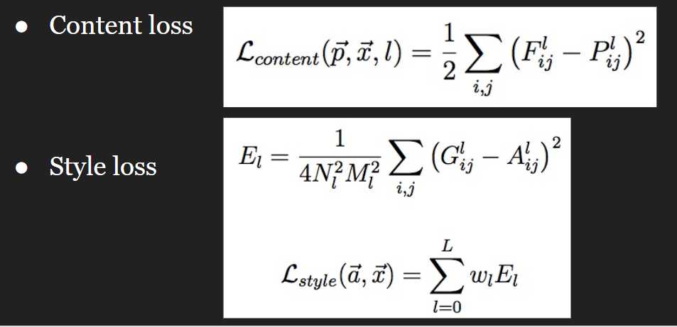
解释:
content loss:
style loss:
(1) N is the third dimension of the feature map(应该是W x H x C,这里N代替C), and M is the product of the first two dimensions of the feature map. However, remember that in TensorFlow, we have to add one extra dimension to make it 4D(也就是batch_size x W x H x C) to make it work for the function tf.nn.conv2d, so the first dimension is actually the second, and the second is the third, and so on.
(2) A is the Gram matrix from the original image and G is the Gram matrix of the image to be generated. To obtain the gram matrix, for example, of the style image, we first need to get the feature map of the style image at that layer, then reshape it to 2D tensor of dimension M x N, and take the dot product of 2D tensor with its transpose.
关于gram matrix的介绍:
(3) 第二个公式小写的L即l,指的是 the layer whose feature maps we want to incorporate into the generated images. In the paper, it suggests that we use feature maps from 5 layers:
[‘conv1_1‘, ‘conv2_1‘, ‘conv3_1‘, ‘conv4_1‘, ‘conv5_1‘]
本论文中,图像的style用gram matrix来表示
(4) After you’ve calculated the tensors E’s, you calculate the style loss by summing them up with their corresponding weight w’s. You can tune w’s, but I’d suggest that you give more emphasis to deep layers. For example, w for ‘conv1_1’ can be 1, then weight for ‘conv2_1’ can be 2, and so on. (因为一般认为,style在 deeper layer中更显著)
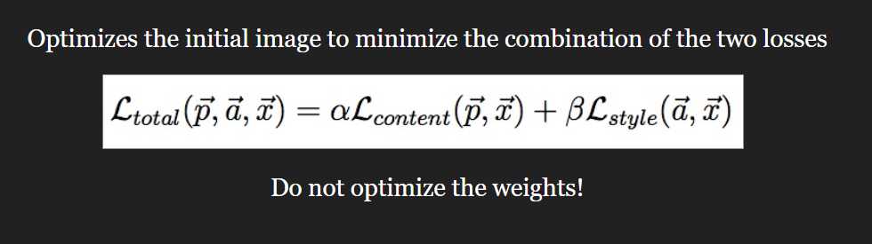
total_loss
注意:不要优化weights (谁的weights ?)- TODO
Tricky implementation details
Train input instead of weights
Multiple tensors share the same variable to avoid assembling identical subgraphs
Use pre-trained weights (from VGG-19)
本实验3个特点:
For this model, you have two fixed inputs: content image and style image, but also have a trainable input which will be trained to become the generated artwork. (but weights fixed)
There is not a clear distinction between the two phases of a TensorFlow program: assembling the graph and executing it. All the 3 input (content image, style image, and trainable input) have the same dimensions and act as input to the same computation to extract the same sets of features. To save us from having to assemble the same subgraph multiple times, we will use one variable for all three of them. The variable is already defined for you in the model as:
self.input_img = tf.get_variable('in_img',
                             shape=([1, self.img_height, self.img_width, 3]),
                             dtype=tf.float32,
                             initializer=tf.zeros_initializer())
When we need to do some computation that takes in the content image as the input, we first assign the content image to that variable, and so on.(还有 style img, trainable input), 三张图片在不同时刻分别给同一个variable赋值
tranfer learning:
we use the weights trained for another task for this task. We will use the weights and biases already trained for the object recognition task of the model VGG-19 (a convolutional network with 19 layers) to extract content and style layers for style transfer. We’ll only use their weights for the convolution layers. The paper by Gatys et al. suggested that average pooling is better than max pooling, so we’ll have to do pooling ourselves.
回顾一个基本的model pipeline
Step 1: Define inference
Step 2: Create loss functions
Step 3: Create optimizer
Step 4: Create summaries to monitor your training process
Step 5: Train your model
几个重点
loss的分析及实践细节:上面已经论述了
optimizer的选择:
I suggest AdamOptimizer but you can be creative with both optimizers and learning rate to see what you find. You can find this part in the optimize() method in style_transfer.py.
注意跟踪实验过程
The training curve of content loss, style loss, and the total loss. Write a few sentences about what you see. (一定一定多用summary, tensorboard)
The graph of your model. (by tensorboard)
Change at least two parameters, explain what you did and how that changed the results. (这种实验加解释实验结果,就是科研的过程)
3 artworks generated using at least 3 different styles. (至少使用3个style image)
参考:
下载VGG19的预训练结果并加载到本model中
下载 .mat文件:http://www.vlfeat.org/matconvnet/models/imagenet-vgg-verydeep-19.mat
.mat文件对应的网络:http://www.vlfeat.org/matconvnet/models/imagenet-vgg-verydeep-19.svg
只有分析清楚了网络结构,才能加载并处理预训练结果,本mat文件的网络具体结构(VGG19)的基本结构(从vgg19.svg计算图的角度来看)如下:
| layer_name | idx (即在forzen.mat中layer index) | shape_w | shape_b |
|---|---|---|---|
| conv1_1 | 0 | 3x3x3x64 | 64x1 |
| relu1_1 | 1 | ||
| conv1_2 | 2 | 3x3x64x64 | 64x1 |
| relu_1_2 | 3 | ||
| pool1 | 4 | ||
| conv2_1 | 5 | 3x3x64x128 | 128x1 |
| relu2_1 | 6 | ||
| conv2_2 | 7 | 3x3x128x128 | 128x1 |
| relu2_2 | 8 | ||
| pool2 | 9 | ||
| conv3_1 | 10 | 3x3x128x256 | 256x1 |
| relu3_1 | 11 | ||
| conv3_2 | 12 | 3x3x256x256 | 256x1 |
| relu3_2 | 13 | ||
| conv3_3 | 14 | 3x3x256x256 | 256x1 |
| relu3_3 | 15 | ||
| conv3_4 | 16 | 3x3x256x256 | 256x1 |
| relu3_4 | 17 | ||
| pool3 | 18 | ||
| conv4_1 | 19 | 3x3x256x512 | 512x1 |
| relu4_1 | 20 | ||
| conv4_2 | 21 | 3x3x512x512 | 512x1 |
| relu4_2 | 22 | ||
| conv4_3 | 23 | 3x3x512x512 | 512x1 |
| relu4_3 | 24 | ||
| conv4_4 | 25 | 3x3x512x512 | 512x1 |
| relu4_4 | 26 | ||
| pool4 | 27 | ||
| conv5_1 | 28 | 3x3x512x512 | 512x1 |
| relu5_1 | 29 | ||
| conv5_2 | 30 | 3x3x512x512 | 512x1 |
| relu5_2 | 31 | ||
| conv5_3 | 32 | 3x3x512x512 | 512x1 |
| relu5_3 | 33 | ||
| conv5_4 | 34 | 3x3x512x512 | 512x1 |
| relu5_4 | 35 | ||
| pool5 | 36 | ||
| fc6 | 37 | 7x7x512x4096 | 4096x1 |
| relu6 | 38 | ||
| fc7 | 39 | 1x1x4096x4096 | 4096x1 |
| relu7 | 40 | ||
| fc8 | 41 | 1x1x4096x1000 | 1000x1 |
| prob | 42 |
python处理mat格式文件:https://blog.csdn.net/google19890102/article/details/45672305
# 测试下 vgg19.mat的结构,其实很复杂,还是要参考官方对于vgg19.mat的解释以及我自己对于vgg19的已有认知
def test_1():
    # 测试下vgg19的结构
    import A2_utils
    import scipy.io

    # VGG-19 parameters file
    VGG_DOWNLOAD_LINK = 'http://www.vlfeat.org/matconvnet/models/imagenet-vgg-verydeep-19.mat'
    VGG_FILENAME = 'imagenet-vgg-verydeep-19.mat'
    EXPECTED_BYTES = 534904783
    A2_utils.download(VGG_DOWNLOAD_LINK, VGG_FILENAME, EXPECTED_BYTES)
    vgg19 = scipy.io.loadmat(VGG_FILENAME)
    #
    print("vgg19-keys: ", vgg19.keys())
    layers = vgg19['layers']
    # print("vgg19-layers: ", layers)
    # dict_keys(['__header__', '__version__', '__globals__', 'layers', 'meta'])
    #
    print("vgg19-layers-type: ", type(layers)) # <class 'numpy.ndarray'>
    #
    print("数组元素数据类型:", layers.dtype)  # object
    print("数组元素总数:", layers.size)  # 43 //结合vgg19.svg,刚好是43个计算图节点(0-42)
    print("数组形状:", layers.shape)  # (1, 43)
    print("数组的维度数目", layers.ndim)  # 2
    #
    print("应该是 pool: ", layers[0][4])
    # [[(array(['pool1'], dtype='<U5'), array(['pool'], dtype='<U4'), array()...]]
    print("应该是 conv2_1: ", layers[0][5])
    # [[ (array(['conv2_1'], dtype='<U7'),
    #     array(['conv'], dtype='<U4'),
    #     array([[array([[[[-2.40122317e-03, ...]])
    #     ....
    # ]]
    print("应该是 prob: ", layers[0][42])   #
    # 上面测试的实际与预料符合
    #
    # print("vgg19-meta: ", vgg19['meta'])
    #
    # print(vgg19)
test_1()
上述测试代码运行结果
vgg19-keys:  dict_keys(['__header__', '__version__', '__globals__', 'layers', 'meta'])

# 'layers': 43个计算图节点的信息,但是每个节点的结构比较复杂,特别是conv op,根据w/b的shape会有较大的shape,还是要参考官方文档才能正确使用

# 'meta': 从打印信息,看不出来,但我类比tensorflow的xxx.meta文件,猜这个是 meta-graph
注意事项
avgpool5有一部分的loss 编码无法理解,TODO,见代码的 TODO部分
标签:one 控制 when scalar oar 下载 instead between var
原文地址:https://www.cnblogs.com/LS1314/p/10371215.html