标签:and 零极点 git mod man art hit col 脉冲
代码:
%% ------------------------------------------------------------------------
%%            Output Info about this m-file
fprintf(‘\n***********************************************************\n‘);
fprintf(‘        <DSP using MATLAB> Problem 8.10 \n\n‘);
banner();
%% ------------------------------------------------------------------------

%a0 = 0.90;
%a0 = 0.95;
a0 = 0.99;
% digital iir 1st-order allpass filter
b = [a0  1];
a = [1  a0];

figure(‘NumberTitle‘, ‘off‘, ‘Name‘, ‘Problem 8.10 Pole-Zero Plot‘)
set(gcf,‘Color‘,‘white‘);
zplane(b,a);
title(sprintf(‘Pole-Zero Plot, r=%.2f‘,a0));
%pzplotz(b,a);

[db, mag, pha, grd, w] = freqz_m(b, a);

% ---------------------------------------------------------------------
%  Choose the gain parameter of the filter, maximum gain is equal to 1
% ---------------------------------------------------------------------
gain1=max(mag)                    % with poles
K = 1
[db, mag, pha, grd, w] = freqz_m(K*b, a);

figure(‘NumberTitle‘, ‘off‘, ‘Name‘, ‘Problem 8.10 IIR allpass filter‘)
set(gcf,‘Color‘,‘white‘);

subplot(2,2,1); plot(w/pi, db); grid on; axis([0 2 -60 10]);
set(gca,‘YTickMode‘,‘manual‘,‘YTick‘,[-60,-30,0])
set(gca,‘YTickLabelMode‘,‘manual‘,‘YTickLabel‘,[‘60‘;‘30‘;‘ 0‘]);
set(gca,‘XTickMode‘,‘manual‘,‘XTick‘,[0,0.25,0.5,1,1.5,1.75,2]);
xlabel(‘frequency in \pi units‘); ylabel(‘Decibels‘); title(‘Magnitude Response in dB‘);

subplot(2,2,3); plot(w/pi, mag); grid on; %axis([0 1 -100 10]);
xlabel(‘frequency in \pi units‘); ylabel(‘Absolute‘); title(‘Magnitude Response in absolute‘);
set(gca,‘XTickMode‘,‘manual‘,‘XTick‘,[0,0.25,0.5,1,1.5,1.75,2]);
set(gca,‘YTickMode‘,‘manual‘,‘YTick‘,[0,1.0]);

subplot(2,2,2); plot(w/pi, pha); grid on; %axis([0 1 -100 10]);
xlabel(‘frequency in \pi units‘); ylabel(‘Rad‘); title(‘Phase Response in Radians‘);

subplot(2,2,4); plot(w/pi, grd*pi/180);  grid on; %axis([0 1 -100 10]);
xlabel(‘frequency in \pi units‘); ylabel(‘Rad‘); title(‘Group Delay‘);
set(gca,‘XTickMode‘,‘manual‘,‘XTick‘,[0,0.25,0.5,1,1.5,1.75,2]);
%set(gca,‘YTickMode‘,‘manual‘,‘YTick‘,[0,1.0]);


figure(‘NumberTitle‘, ‘off‘, ‘Name‘, ‘Problem 8.10 IIR allpass filter‘)
set(gcf,‘Color‘,‘white‘);
plot(w/pi, -pha/w); grid on; %axis([0 1 -100 10]);
xlabel(‘frequency in \pi units‘); ylabel(‘Rad‘); title(‘Phase Delay in samples‘);


% Impulse Response
fprintf(‘\n----------------------------------‘);
fprintf(‘\nPartial fraction expansion method: \n‘);
[R, p, c] = residuez(K*b,a)
MR = (abs(R))‘              % Residue  Magnitude
AR = (angle(R))‘/pi         % Residue  angles in pi units
Mp = (abs(p))‘              % pole  Magnitude
Ap = (angle(p))‘/pi         % pole  angles in pi units
[delta, n] = impseq(0,0,50);
h_chk = filter(K*b,a,delta);      % check sequences


% ------------------------------------------------------------------------------------------------
%                                gain parameter K
% ------------------------------------------------------------------------------------------------
%h =  -0.2111 * ((-0.9) .^ n) + 1.1111 * delta;    %r=0.90
%h =  -0.1026 * ((-0.95) .^ n) + 1.0526 * delta;    %r=0.95
h =  -0.0201 * ((-0.99) .^ n) + 1.0101 * delta;    %r=0.99
% ------------------------------------------------------------------------------------------------


figure(‘NumberTitle‘, ‘off‘, ‘Name‘, ‘Problem 8.10 IIR allpass filter, h(n) by filter and Inv-Z ‘)
set(gcf,‘Color‘,‘white‘);

subplot(2,1,1); stem(n, h_chk); grid on; %axis([0 2 -60 10]);
xlabel(‘n‘); ylabel(‘h\_chk‘); title(‘Impulse Response sequences by filter‘);

subplot(2,1,2); stem(n, h); grid on; %axis([0 1 -100 10]);
xlabel(‘n‘); ylabel(‘h‘); title(‘Impulse Response sequences by Inv-Z‘);


[db, mag, pha, grd, w] = freqz_m(h, 1);


figure(‘NumberTitle‘, ‘off‘, ‘Name‘, ‘Problem 8.10 IIR filter, h(n) by Inv-Z ‘)
set(gcf,‘Color‘,‘white‘);

subplot(2,2,1); plot(w/pi, db); grid on; axis([0 2 -60 10]);
set(gca,‘YTickMode‘,‘manual‘,‘YTick‘,[-60,-30,0])
set(gca,‘YTickLabelMode‘,‘manual‘,‘YTickLabel‘,[‘60‘;‘30‘;‘ 0‘]);
set(gca,‘XTickMode‘,‘manual‘,‘XTick‘,[0,0.25,1,1.75,2]);
xlabel(‘frequency in \pi units‘); ylabel(‘Decibels‘); title(‘Magnitude Response in dB‘);

subplot(2,2,3); plot(w/pi, mag); grid on; %axis([0 1 -100 10]);
xlabel(‘frequency in \pi units‘); ylabel(‘Absolute‘); title(‘Magnitude Response in absolute‘);
set(gca,‘XTickMode‘,‘manual‘,‘XTick‘,[0,0.25,1,1.75,2]);
set(gca,‘YTickMode‘,‘manual‘,‘YTick‘,[0,1.0]);

subplot(2,2,2); plot(w/pi, pha); grid on; %axis([0 1 -100 10]);
xlabel(‘frequency in \pi units‘); ylabel(‘Rad‘); title(‘Phase Response in Radians‘);

subplot(2,2,4); plot(w/pi, grd*pi/180);  grid on; %axis([0 1 -100 10]);
xlabel(‘frequency in \pi units‘); ylabel(‘Rad‘); title(‘Group Delay‘);
set(gca,‘XTickMode‘,‘manual‘,‘XTick‘,[0,0.25,1,1.75,2]);
%set(gca,‘YTickMode‘,‘manual‘,‘YTick‘,[0,1.0]);
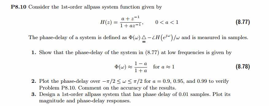
运行结果:
第1、2小题的图这里不放了。
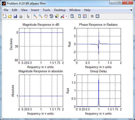
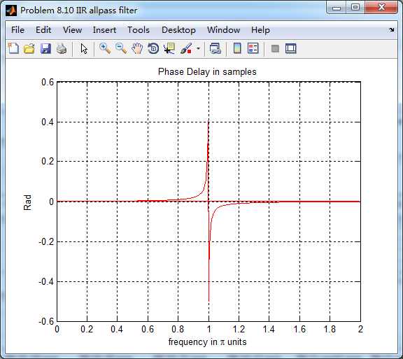
相位延迟phase-delay为0.01时对应的a 的值0.9802
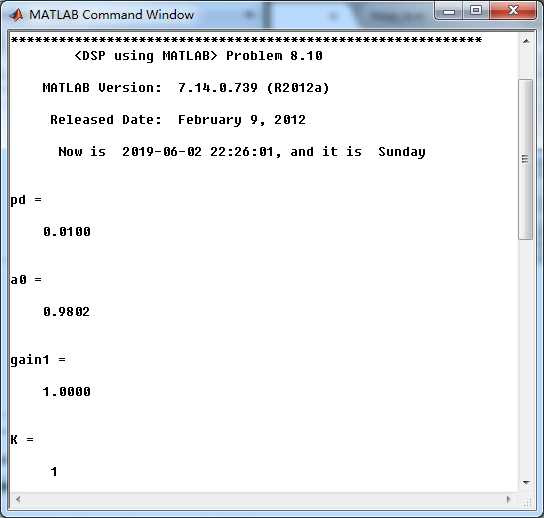
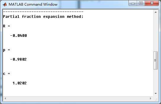
此时1阶全通系统的留数、极点为
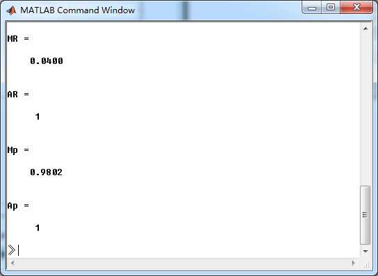
系统零极点图
该系统部分分式展开后,求逆z变换得脉冲响应
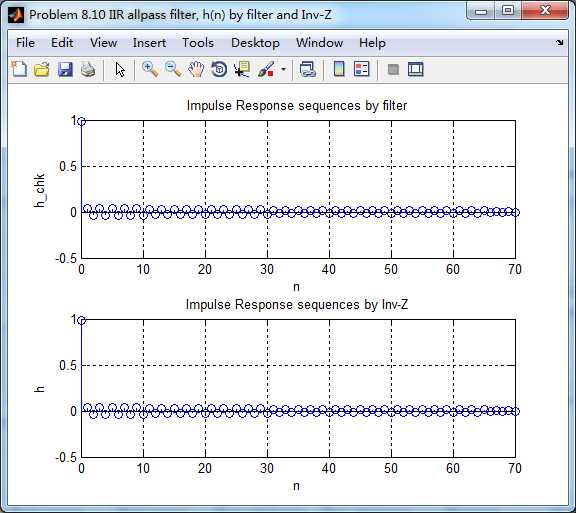
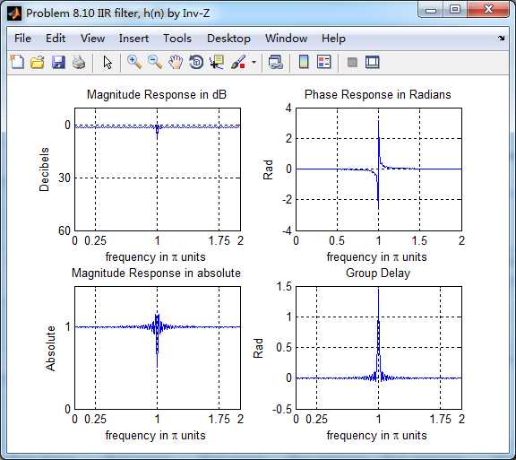
由下图知,两种方法得到的系统脉冲响应h的幅度谱、相位谱、群延迟大致类似(ω=π时不同)。
《DSP using MATLAB》Problem 8.10
标签:and 零极点 git mod man art hit col 脉冲
原文地址:https://www.cnblogs.com/ky027wh-sx/p/11001129.html