标签:rom 国产 次数 ase 结果 key apt 江湖 analysis
获取到数据之后,首先对用户location做可视化
第一步 做数据清洗,把里面的数据中文符号全部转为为空格
import re
f = open(‘name.txt‘,‘r‘)
for line in f.readlines():
        string = re.sub("[\s+\.\!\/_,$%^*(+\"\‘]+|[+——!,。?、~@#¥%……&*()]+", " ", line)
        print(line)
        print(string)
        f1=open("newname.txt",‘a‘,encoding=‘utf-8‘)
        f1.write(string)
        f1.close()
f.close()
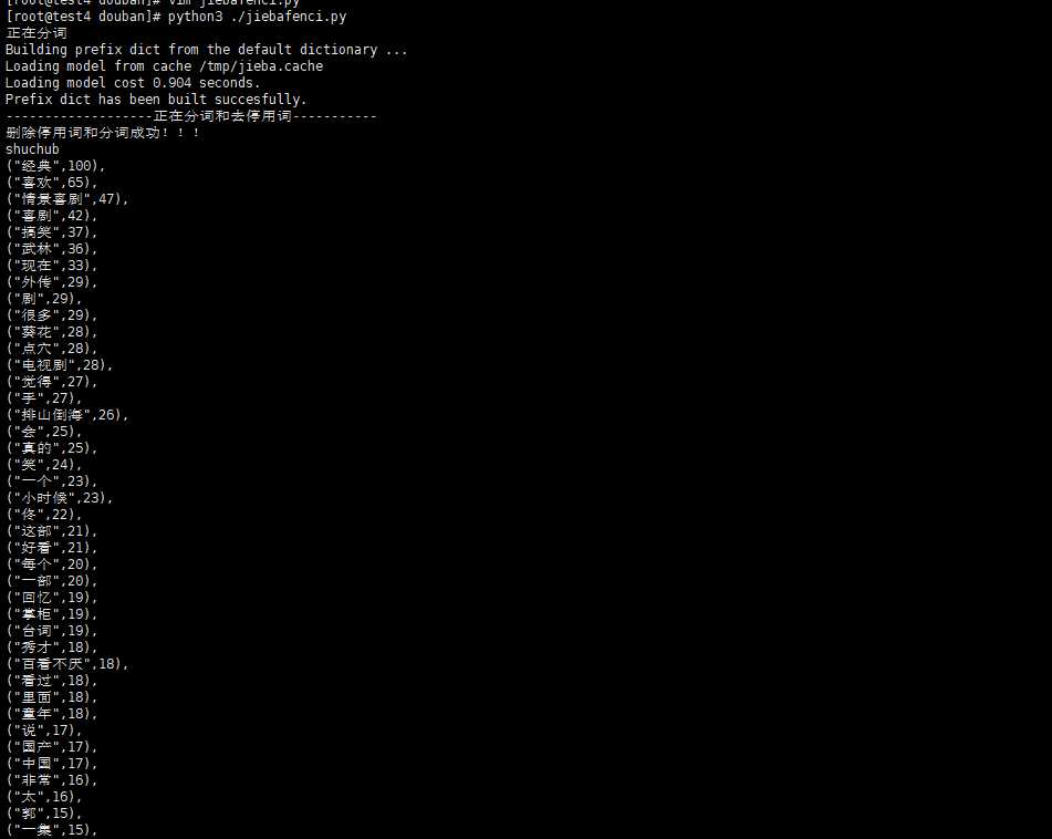
第二步 数据做词云,需要过滤停用词,然后分词
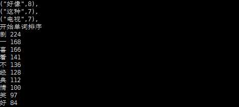
#定义结巴分词的方法以及处理过程
import jieba.analyse
import jieba

#需要输入需要分析的文本名称,分析后输入的文本名称
class worldAnalysis():
    def __init__(self,inputfilename,outputfilename):
        self.inputfilename=inputfilename
        self.outputfilename=outputfilename
        self.start()
#--------------------------------这里实现分词和去停用词---------------------------------------
# 创建停用词列表
    def stopwordslist(self):
        stopwords = [line.strip() for line in open(‘ting.txt‘,encoding=‘UTF-8‘).readlines()]
        return stopwords

    # 对句子进行中文分词
    def seg_depart(self,sentence):
        # 对文档中的每一行进行中文分词
        print("正在分词")
        sentence_depart = jieba.cut(sentence.strip())
        # 创建一个停用词列表
        stopwords = self.stopwordslist()
        # 输出结果为outstr
        outstr = ‘‘
        # 去停用词
        for word in sentence_depart:
            if word not in stopwords:
                if word != ‘\t‘:
                    outstr += word
                    outstr += " "
        return outstr

    def start(self):
        # 给出文档路径
        filename = self.inputfilename
        outfilename = self.outputfilename
        inputs = open(filename, ‘r‘, encoding=‘UTF-8‘)
        outputs = open(outfilename, ‘w‘, encoding=‘UTF-8‘)

        # 将输出结果写入ou.txt中
        for line in inputs:
            line_seg = self.seg_depart(line)
            outputs.write(line_seg + ‘\n‘)
            print("-------------------正在分词和去停用词-----------")
        outputs.close()
        inputs.close()
        print("删除停用词和分词成功!!!")

        self.LyricAnalysis()

    #实现数据词频统计
    def splitSentence(self):
        #下面的程序完成分析前十的数据出现的次数
        f = open(self.outputfilename, ‘r‘, encoding=‘utf-8‘)
        a = f.read().split()
        b = sorted([(x, a.count(x)) for x in set(a)], key=lambda x: x[1], reverse=True)
        #print(sorted([(x, a.count(x)) for x in set(a)], key=lambda x: x[1], reverse=True))
        print("shuchub")
#        for i in range(0,100):
#               print(b[i][0],end=‘,‘)
#        print("---------")
#        for i in range(0,100):
#               print(b[i][1],end=‘,‘)
        for i in range(0,100):
            print("("+‘"‘+b[i][0]+‘"‘+","+ str(b[i][1])+‘)‘+‘,‘)

    #输出频率最多的前十个字,里面调用splitSentence完成频率出现最多的前十个词的分析
    def LyricAnalysis(self):
        import jieba
        file = self.outputfilename
        #这个技巧需要注意
        alllyric = str([line.strip() for line in open(file,encoding="utf-8").readlines()])
    #获取全部歌词,在一行里面
        alllyric1=alllyric.replace("‘","").replace(" ","").replace("?","").replace(",","").replace(‘"‘,‘‘).replace("?","").replace(".","").replace("!","").replace(":","")
       # print(alllyric1)
        self.splitSentence()
        #下面是词频(单个汉字)统计
        import collections
        # 读取文本文件,把所有的汉字拆成一个list
        f = open(file, ‘r‘, encoding=‘utf8‘)  # 打开文件,并读取要处理的大段文字
        txt1 = f.read()
        txt1 = txt1.replace(‘\n‘, ‘‘)  # 删掉换行符
        txt1 = txt1.replace(‘ ‘, ‘‘)  # 删掉换行符
        txt1 = txt1.replace(‘.‘, ‘‘)  # 删掉逗号
        txt1 = txt1.replace(‘.‘, ‘‘)  # 删掉句号
        txt1 = txt1.replace(‘o‘, ‘‘)  # 删掉句号
        mylist = list(txt1)
        mycount = collections.Counter(mylist)
        for key, val in mycount.most_common(10):  # 有序(返回前10个)
            print("开始单词排序")
            print(key, val)
#输入文本为 newcomment.txt 输出 test.txt
AAA=worldAnalysis("newcomment.txt","test.txt")
输入结果 这样输出的原因是后面需要用pyechart做数据的词云
第三步 词云可视化
from pyecharts import options as opts
from pyecharts.charts import Page, WordCloud
from pyecharts.globals import SymbolType
from pyecharts.charts import Bar

from pyecharts.render import make_snapshot
from snapshot_selenium import snapshot

words = [
("经典",100),
("喜欢",65),
("情景喜剧",47),
("喜剧",42),
("搞笑",37),
("武林",36),
("现在",33),
("剧",29),
("外传",29),
("很多",29),
("点穴",28),
("葵花",28),
("电视剧",28),
("手",27),
("觉得",27),
("排山倒海",26),
("真的",25),
("会",25),
("笑",24),
("一个",23),
("小时候",23),
("佟",22),
("好看",21),
("这部",21),
("一部",20),
("每个",20),
("掌柜",19),
("台词",19),
("回忆",19),
("看过",18),
("里面",18),
("百看不厌",18),
("童年",18),
("秀才",18),
("国产",17),
("说",17),
("中国",17),
("太",16),
("非常",16),
("一集",15),
("郭",15),
("宁财神",15),
("没有",15),
("不错",14),
("不会",14),
("道理",14),
("重温",14),
("挺",14),
("演员",14),
("爱",13),
("中",13),
("哈哈哈",13),
("人生",13),
("老白",13),
("人物",12),
("故事",12),
("集",12),
("情景剧",11),
("开心",11),
("感觉",11),
("之后",11),
("点",11),
("时",11),
("幽默",11),
("每次",11),
("角色",10),
("完",10),
("里",10),
("客栈",10),
("看看",10),
("发现",10),
("生活",10),
("江湖",10),
("~",10),
("记得",10),
("起来",9),
("特别",9),
("剧情",9),
("一直",9),
("一遍",9),
("印象",9),
("看到",9),
("不好",9),
("当时",9),
("最近",9),
("欢乐",9),
("知道",9),
("芙蓉",8),
("之作",8),
("绝对",8),
("无法",8),
("十年",8),
("依然",8),
("巅峰",8),
("好像",8),
("长大",8),
("深刻",8),
("无聊",8),
("以前",7),
("时间",7),

]


def wordcloud_base() -> WordCloud:
    c = (
        WordCloud()
        .add("", words, word_size_range=[20, 100],shape="triangle-forward",)
        .set_global_opts(title_opts=opts.TitleOpts(title="WordCloud-基本示例"))
    )
    return c
make_snapshot(snapshot, wordcloud_base().render(), "bar.png")
# wordcloud_base().render()

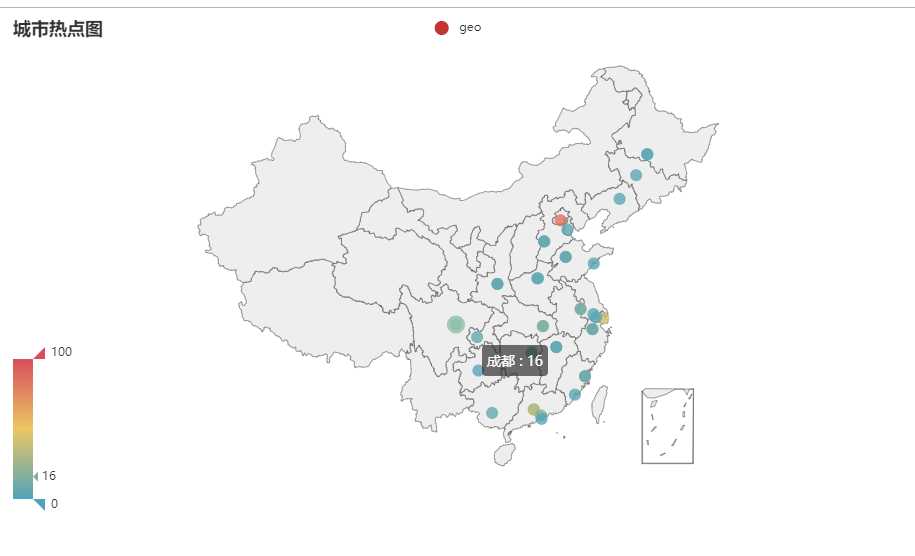
二 用户地址可视化

用户所在地成都热点图
程序脚本:这里需要注意这里的城市一定要是中国城市的名称,为了处理元数据用了xlml(f)+py 随便放一下py脚本
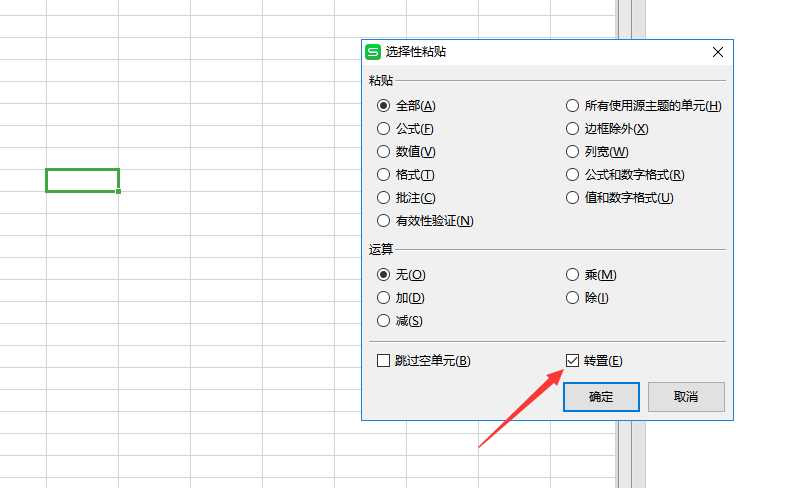
数据处理

f=open("city.txt",‘r‘)
for i in f.readlines():
        #print(i,end=",")
        print(‘"‘+i.strip()+‘"‘,end=",")
from example.commons import Faker
from pyecharts import options as opts
from pyecharts.charts import Geo
from pyecharts.globals import ChartType, SymbolType

def geo_base() -> Geo:
    c = (
        Geo()
        .add_schema(maptype="china")
        .add("geo", [list(z) for z in zip(["北京","广东","上海","广州","江苏","四川","武汉","湖北","深圳","成都","浙江","山东","福建","南京","福州","河北","江西","南宁","杭州","湖南","长沙","河南","郑州","苏州","重庆","济南","黑龙江","石家庄","西安","南昌","陕西","哈尔滨","吉林","厦门","天津","沈阳","香港","青岛","无锡","贵州"], ["86","52","42","29","26","20","16","16","16","16","13","12","12","12","8","7","7","7","7","6","6","6","6","6","6","6","5","5","5","5","5","5","4","4","4","4","3","3","3","3"])])
        .set_series_opts(label_opts=opts.LabelOpts(is_show=False))
        .set_global_opts(
            visualmap_opts=opts.VisualMapOpts(),
            title_opts=opts.TitleOpts(title="城市热点图"),
        )
    )
    return c
geo_base().render()
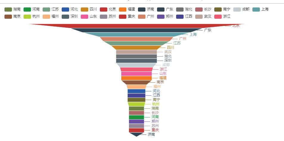
漏斗图 由于页面适配的问题这里已经筛减了很多城市了
from example.commons import Faker
from pyecharts import options as opts
from pyecharts.charts import Funnel, Page


def funnel_base() -> Funnel:
    c = (
        Funnel()
            .add("geo", [list(z) for z in zip(
            ["北京", "广东", "上海", "广州", "江苏", "四川", "武汉", "湖北", "深圳", "成都", "浙江", "山东", "福建", "南京", "福州", "河北", "江西", "南宁",
             "杭州", "湖南", "长沙", "河南", "郑州", "苏州", "重庆", "济南"],
            ["86", "52", "42", "29", "26", "20", "16", "16", "16", "16", "13", "12", "12", "12", "8", "7", "7", "7",
             "7", "6", "6", "6", "6", "6", "6", "6"])])

            .set_global_opts(title_opts=opts.TitleOpts())
    )
    return c
funnel_base().render(‘漏斗图.html‘)
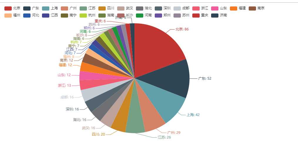
饼图
from example.commons import Faker
from pyecharts import options as opts
from pyecharts.charts import Page, Pie


def pie_base() -> Pie:
    c = (
        Pie()
        .add("", [list(z) for z in zip(  ["北京", "广东", "上海", "广州", "江苏", "四川", "武汉", "湖北", "深圳", "成都", "浙江", "山东", "福建", "南京", "福州", "河北", "江西", "南宁",
             "杭州", "湖南", "长沙", "河南", "郑州", "苏州", "重庆", "济南"],
            ["86", "52", "42", "29", "26", "20", "16", "16", "16", "16", "13", "12", "12", "12", "8", "7", "7", "7",
             "7", "6", "6", "6", "6", "6", "6", "6"])])
        .set_global_opts(title_opts=opts.TitleOpts())
        .set_series_opts(label_opts=opts.LabelOpts(formatter="{b}: {c}"))
    )
    return c

pie_base().render("饼图.html")
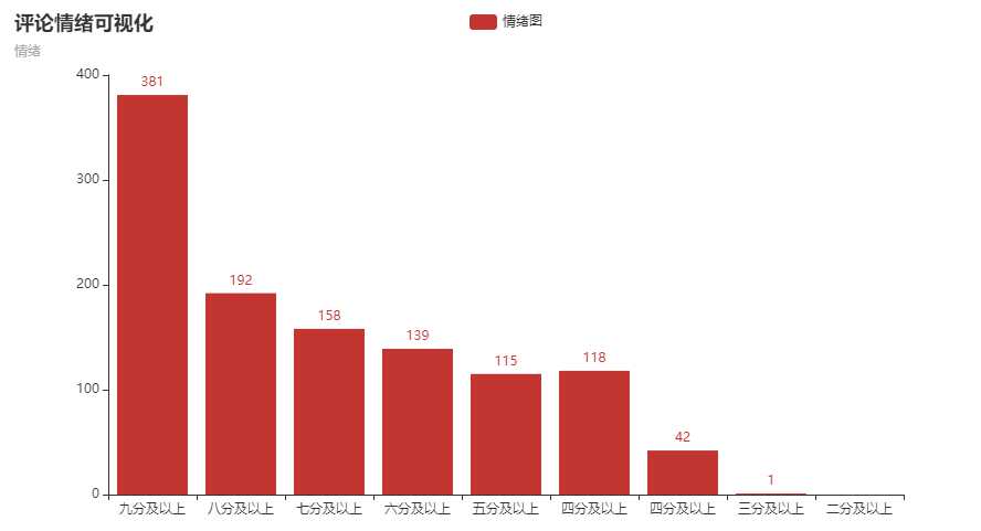
评论情绪化分析代码如下
from snownlp import SnowNLP
f=open("comment.txt",‘r‘)
sentiments=0
count=0

point2=0
point3=0
point4=0
point5=0
point6=0
point7=0
point8=0
point9=0
for i in f.readlines():
        s = SnowNLP(i)
        s1 = SnowNLP(s.sentences[0])
        for p in s.sentences:
                s = SnowNLP(p)
                s1 = SnowNLP(s.sentences[0])
                count+=1
                if s1.sentiments > 0.9:
                        point9+=1
                elif s1.sentiments> 0.8 and s1.sentiments <=0.9:
                        point8+=1
                elif s1.sentiments> 0.7 and s1.sentiments <=0.8:
                        point7+=1
                elif s1.sentiments> 0.6 and s1.sentiments <=0.7:
                        point6+=1
                elif s1.sentiments> 0.5 and s1.sentiments <=0.6:
                        point5+=1
                elif s1.sentiments> 0.4 and s1.sentiments <=0.5:
                        point4+=1
                elif s1.sentiments> 0.3 and s1.sentiments <=0.4:
                        point3+=1
                elif s1.sentiments> 0.2 and s1.sentiments <=0.3:
                        point2=1
                print(s1.sentiments)
                sentiments+=s1.sentiments

print(sentiments)
print(count)
avg1=int(sentiments)/int(count)
print(avg1)


print(point9)
print(point8)
print(point7)
print(point6)
print(point5)
print(point4)
print(point3)
print(point2)
情绪可视化
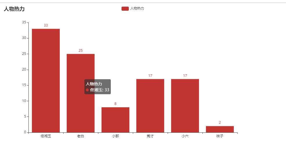
主要人物热力图
cat comment.txt  | grep -E  ‘佟|掌柜|湘玉|闫妮‘  | wc -l
33
cat comment.txt  | grep -E  ‘老白|展堂|盗圣‘  | wc -l
25
cat comment.txt  | grep -E  ‘大嘴‘  | wc -l
8
cat comment.txt  | grep -E  ‘小郭|郭|芙蓉‘  | wc -l
17
cat comment.txt  | grep -E  ‘秀才|吕轻侯‘  | wc -l
17
cat comment.txt  | grep -E  ‘小六‘  | wc -l
2
from pyecharts.charts import Bar
from pyecharts import options as opts

# V1 版本开始支持链式调用
bar = (
    Bar()
    .add_xaxis(["佟湘玉", "老白", "小郭", "秀才", "小六", "袜子"])
    .add_yaxis("人物热力", [33, 25, 8, 17, 17, 2])
    .set_global_opts(title_opts=opts.TitleOpts(title="人物热力"))
    # 或者直接使用字典参数
    # .set_global_opts(title_opts={"text": "主标题", "subtext": "副标题"})
)
bar.render("人物热力.html")
标签:rom 国产 次数 ase 结果 key apt 江湖 analysis
原文地址:https://www.cnblogs.com/ZFBG/p/11051116.html