标签:title 模拟 his inf for elm Plan lan img
10月1日,新中国70周岁生日,上午观看了盛大的庆祝仪式,整齐的方阵,先进的武器,尊敬的先辈英雄,欢乐的人们,愿我们的
国家越来越好,人民生活越来越好。
接着做题。
代码:
%% ------------------------------------------------------------------------
%%            Output Info about this m-file
fprintf(‘\n***********************************************************\n‘);
fprintf(‘        <DSP using MATLAB> Problem 8.30 \n\n‘);

banner();
%% ------------------------------------------------------------------------

% -----------------------------------
%          Ω=(2/T)tan(ω/2)
%          ω=2*[atan(ΩT/2)]
%    Digital Filter Specifications:
% -----------------------------------
wp = 0.4*pi;                     % digital passband freq in rad
ws = 0.6*pi;                     % digital stopband freq in rad
Rp = 0.5;                        % passband ripple in dB
As = 50;                         % stopband attenuation in dB

Ripple = 10 ^ (-Rp/20)           % passband ripple in absolute
Attn = 10 ^ (-As/20)             % stopband attenuation in absolute

% Analog prototype specifications: Inverse Mapping for frequencies
T = 2;                           % set T = 1
Fs = 1/T;
OmegaP = (2/T)*tan(wp/2);        % prototype passband freq
OmegaS = (2/T)*tan(ws/2);        % prototype stopband freq

% Analog Butterworth Prototype Filter Calculation:
[cs, ds] = afd_butt(OmegaP, OmegaS, Rp, As);

% Calculation of second-order sections:
fprintf(‘\n***** Cascade-form in s-plane: START *****\n‘);
[CS, BS, AS] = sdir2cas(cs, ds);
fprintf(‘\n***** Cascade-form in s-plane: END *****\n‘);

% Calculation of Frequency Response:
[db_s, mag_s, pha_s, ww_s] = freqs_m(cs, ds, 2*pi/T);


% --------------------------------------------------------------------
%   find exact band-edge frequencies for the given dB specifications
% --------------------------------------------------------------------
%ind = find( abs(ceil(db_s))-50 == 0 )
[diff_to_50dB, ind] = min(abs(db_s+50))
db_s(ind-3 : ind+3)                                     % magnitude response, dB

ww_s(ind)/(pi)          % analog frequency in kpi units
%ww_s(ind)/(2*pi)        % analog frequency in Hz units

[sA,index] = sort(abs(db_s+50));
AA_dB = db_s(index(1:8))
AB_rad = ww_s(index(1:8))/(pi)
AC_Hz = ww_s(index(1:8))/(2*pi)
% -------------------------------------------------------------------


% Calculation of Impulse Response:
[ha, x, t] = impulse(cs, ds);


% Impulse Invariance Transformation:
%[b, a] = imp_invr(cs, ds, T);

% Bilinear Transformation
[b, a] = bilinear(cs, ds, Fs);
[C, B, A] = dir2cas(b, a);

% Calculation of Frequency Response:
[db, mag, pha, grd, ww] = freqz_m(b, a);

% --------------------------------------------------------------------
%   find exact band-edge frequencies for the given dB specifications
% --------------------------------------------------------------------
%ind = find( abs(ceil(db))-50 == 0 )
[diff_to_80dB, ind] = min(abs(db+50))
db(ind-3 : ind+3)                                     % magnitude response, dB

ww(ind)/(pi)
%ww(ind)*Fs/(2*pi)

(2/T)*tan(ww(ind)/2)/pi

[sA,index] = sort(abs(db+50));
AA_dB = db(index(1:8))‘
AB_rad = ww(index(1:8))‘/pi
AC_Hz = (2/T)*tan(ww(index(1:8))‘/2)/pi
% -------------------------------------------------------------------


%% -----------------------------------------------------------------
%%                             Plot
%% -----------------------------------------------------------------
figure(‘NumberTitle‘, ‘off‘, ‘Name‘, ‘Problem 8.30 Analog Butterworth lowpass‘)
set(gcf,‘Color‘,‘white‘);
M = 1;                          % Omega max

subplot(2,2,1); plot(ww_s/pi, mag_s);  grid on; axis([-M, M, 0, 1.2]);
xlabel(‘ Analog frequency in \pi units‘); ylabel(‘|H|‘); title(‘Magnitude in Absolute‘);
%set(gca, ‘XTickMode‘, ‘manual‘, ‘XTick‘, [-0.876, -0.463, 0, 0.463, 0.876]);        % T=1
set(gca, ‘XTickMode‘, ‘manual‘, ‘XTick‘, [-0.44, -0.23, 0, 0.23, 0.44]);     % T=2
set(gca, ‘YTickMode‘, ‘manual‘, ‘YTick‘, [0, 0.0032, 0.5, 0.9441, 1]);

subplot(2,2,2); plot(ww_s/pi, db_s);  grid on; axis([-M, M, -100, 10]);
xlabel(‘Analog frequency in \pi units‘); ylabel(‘Decibels‘); title(‘Magnitude in dB ‘);
%set(gca, ‘XTickMode‘, ‘manual‘, ‘XTick‘, [-0.876, -0.463, 0, 0.463, 0.8591, 0.876]);        % T=1
set(gca, ‘XTickMode‘, ‘manual‘, ‘XTick‘, [-0.44, -0.23, 0, 0.23, 0.4295, 0.44]);     % T=2
set(gca, ‘YTickMode‘, ‘manual‘, ‘YTick‘, [-90, -50, -1, 0]);
set(gca,‘YTickLabelMode‘,‘manual‘,‘YTickLabel‘,[‘90‘;‘50‘;‘ 1‘;‘ 0‘]);

subplot(2,2,3); plot(ww_s/pi, pha_s/pi);  grid on; axis([-M, M, -1.2, 1.2]);
xlabel(‘Analog frequency in \pi nuits‘); ylabel(‘radians‘); title(‘Phase Response‘);
set(gca, ‘XTickMode‘, ‘manual‘, ‘XTick‘, [-OmegaS, -OmegaP, 0, OmegaP, OmegaS]/pi);
set(gca, ‘YTickMode‘, ‘manual‘, ‘YTick‘, [-1:0.5:1]);

subplot(2,2,4); plot(t, ha); grid on; %axis([0, 30, -0.05, 0.25]);
xlabel(‘time in seconds‘); ylabel(‘ha(t)‘); title(‘Impulse Response‘);


figure(‘NumberTitle‘, ‘off‘, ‘Name‘, ‘Problem 8.30 Digital Butterworth lowpass by afd_butt function‘)
set(gcf,‘Color‘,‘white‘);
M = 2;                          % Omega max

subplot(2,2,1); plot(ww/(pi), mag); axis([0, M, 0, 1.2]); grid on;
xlabel(‘Digital frequency in \pi units‘); ylabel(‘|H|‘); title(‘Magnitude Response‘);
set(gca, ‘XTickMode‘, ‘manual‘, ‘XTick‘, [0, 0.4, 0.6, 1.0, M]);
set(gca, ‘YTickMode‘, ‘manual‘, ‘YTick‘, [0, 0.0032, 0.5, 0.9441, 1]);

subplot(2,2,2); plot(ww/(pi), pha/pi); axis([0, M, -1.1, 1.1]); grid on;
xlabel(‘Digital frequency in \pi nuits‘); ylabel(‘radians in \pi units‘); title(‘Phase Response‘);
set(gca, ‘XTickMode‘, ‘manual‘, ‘XTick‘, [0, 0.4, 0.6, 1.0, M]);
set(gca, ‘YTickMode‘, ‘manual‘, ‘YTick‘, [-1:1:1]);

subplot(2,2,3); plot(ww/pi, db); axis([0, M, -100, 10]); grid on;
xlabel(‘Digital frequency in \pi units‘); ylabel(‘Decibels‘); title(‘Magnitude in dB ‘);
%set(gca, ‘XTickMode‘, ‘manual‘, ‘XTick‘, [0, 0.4, 0.594, 0.6, 1.0, M]);   % T=1
set(gca, ‘XTickMode‘, ‘manual‘, ‘XTick‘, [0, 0.4, 0.594, 0.6, 1.0, M]);   % T=2
set(gca, ‘YTickMode‘, ‘manual‘, ‘YTick‘, [-70, -50, -1, 0]);
set(gca,‘YTickLabelMode‘,‘manual‘,‘YTickLabel‘,[‘70‘;‘50‘;‘ 1‘;‘ 0‘]);

subplot(2,2,4); plot(ww/pi, grd); grid on; %axis([0, M, 0, 35]);
xlabel(‘Digital frequency in \pi units‘); ylabel(‘Samples‘); title(‘Group Delay‘);
set(gca, ‘XTickMode‘, ‘manual‘, ‘XTick‘, [0, 0.4, 0.6, 1.0, M]);
%set(gca, ‘YTickMode‘, ‘manual‘, ‘YTick‘, [0:5:35]);

figure(‘NumberTitle‘, ‘off‘, ‘Name‘, ‘Problem 8.30 Pole-Zero Plot‘)
set(gcf,‘Color‘,‘white‘);
zplane(b,a);
title(sprintf(‘Pole-Zero Plot‘));
%pzplotz(b,a);


% ----------------------------------------------
%       Calculation of Impulse Response
% ----------------------------------------------
figure(‘NumberTitle‘, ‘off‘, ‘Name‘, ‘Problem 8.30 Imp & Freq Response‘)
set(gcf,‘Color‘,‘white‘);
t = [0:0.5:60]; subplot(2,1,1); impulse(cs,ds,t); grid on;   % Impulse response of the analog filter
axis([0,60,-0.3,0.5]);hold on

n = [0:1:60/T]; hn = filter(b,a,impseq(0,0,60/T));           % Impulse response of the digital filter
stem(n*T,hn); xlabel(‘time in sec‘); title (sprintf(‘Impulse Responses, T=%f‘,T));
hold off

% Calculation of Frequency Response:
[dbs, mags, phas, wws] = freqs_m(cs, ds, 2*pi/T);             % Analog frequency   s-domain

[dbz, magz, phaz, grdz, wwz] = freqz_m(b, a);               % Digital  z-domain

%% -----------------------------------------------------------------
%%                             Plot
%% -----------------------------------------------------------------

subplot(2,1,2); plot(wws/(2*pi), mags*Fs,‘b+‘, wwz/(2*pi)*Fs, magz,‘r‘); grid on;

xlabel(‘frequency in Hz‘); title(‘Magnitude Responses‘); ylabel(‘Magnitude‘);

text(-0.3,0.15,‘Analog filter‘, ‘Color‘, ‘b‘); text(0.4,0.55,‘Digital filter‘, ‘Color‘, ‘r‘);


%% +++++++++++++++++++++++++++++++++++++++++++++++++++++++++++++++++++++
%%              MATLAB  butter function
%% +++++++++++++++++++++++++++++++++++++++++++++++++++++++++++++++++++++
% Analog Prototype Order Calculations:
N  = ceil((log10((10^(Rp/10)-1)/(10^(As/10)-1)))/(2*log10(OmegaP/OmegaS)));
fprintf(‘\n\n ********** Butterworth Filter Order = %3.0f  \n‘, N)

OmegaC = OmegaP/((10^(Rp/10)-1)^(1/(2*N)));       % Analog BW prototype cutoff freq
wn = 2*atan((OmegaC*T)/2);                        % Digital BW cutoff freq

% Digital Butterworth Filter Design:
wn = wn/pi;                            % Digital Butterworth cutoff freq in pi units

[b, a] = butter(N, wn); [C, B, A] = dir2cas(b, a)

% Calculation of Frequency Response:
[db, mag, pha, grd, ww] = freqz_m(b, a);

figure(‘NumberTitle‘, ‘off‘, ‘Name‘, ‘Problem 8.30 Digital Butterworth lowpass by butter function‘)
set(gcf,‘Color‘,‘white‘);
M = 2;                          % Omega max

subplot(2,2,1); plot(ww/pi, mag); axis([0, M, 0, 1.2]); grid on;
xlabel(‘ frequency in \pi units‘); ylabel(‘|H|‘); title(‘Magnitude Response‘);
set(gca, ‘XTickMode‘, ‘manual‘, ‘XTick‘, [0, 0.4, 0.6, 1.0, M]);
set(gca, ‘YTickMode‘, ‘manual‘, ‘YTick‘, [0, 0.0032, 0.5, 0.9441, 1]);

subplot(2,2,2); plot(ww/pi, pha/pi); axis([0, M, -1.1, 1.1]); grid on;
xlabel(‘frequency in \pi nuits‘); ylabel(‘radians in \pi units‘); title(‘Phase Response‘);
set(gca, ‘XTickMode‘, ‘manual‘, ‘XTick‘, [0, 0.4, 0.6, 1.0, M]);
set(gca, ‘YTickMode‘, ‘manual‘, ‘YTick‘, [-1:1:1]);

subplot(2,2,3); plot(ww/pi, db); axis([0, M, -100, 10]); grid on;
xlabel(‘frequency in \pi units‘); ylabel(‘Decibels‘); title(‘Magnitude in dB ‘);
set(gca, ‘XTickMode‘, ‘manual‘, ‘XTick‘, [0, 0.4, 0.6, 1.0, M]);
set(gca, ‘YTickMode‘, ‘manual‘, ‘YTick‘, [-70, -50, -1, 0]);
set(gca,‘YTickLabelMode‘,‘manual‘,‘YTickLabel‘,[‘70‘;‘50‘;‘ 1‘;‘ 0‘]);

subplot(2,2,4); plot(ww/pi, grd); grid on; %axis([0, M, 0, 35]);
xlabel(‘frequency in \pi units‘); ylabel(‘Samples‘); title(‘Group Delay‘);
set(gca, ‘XTickMode‘, ‘manual‘, ‘XTick‘, [0, 0.4, 0.6, 1.0, M]);
%set(gca, ‘YTickMode‘, ‘manual‘, ‘YTick‘, [0:5:35]);

figure(‘NumberTitle‘, ‘off‘, ‘Name‘, ‘Problem 8.30 Pole-Zero Plot‘)
set(gcf,‘Color‘,‘white‘);
zplane(b,a);
title(sprintf(‘Pole-Zero Plot‘));
%pzplotz(b,a);


% ----------------------------------------------
%       Calculation of Impulse Response
% ----------------------------------------------
figure(‘NumberTitle‘, ‘off‘, ‘Name‘, ‘Problem 8.30 Imp & Freq Response‘)
set(gcf,‘Color‘,‘white‘);
t = [0:0.5:60]; subplot(2,1,1); impulse(cs,ds,t); grid on;   % Impulse response of the analog filter
axis([0,60,-0.3,0.5]);hold on

n = [0:1:60/T]; hn = filter(b,a,impseq(0,0,60/T));           % Impulse response of the digital filter
stem(n*T,hn); xlabel(‘time in sec‘); title (sprintf(‘Impulse Responses, T=%f‘,T));
hold off

% Calculation of Frequency Response:
[dbs, mags, phas, wws] = freqs_m(cs, ds, 2*pi/T);             % Analog frequency   s-domain

[dbz, magz, phaz, grdz, wwz] = freqz_m(b, a);               % Digital  z-domain

%% -----------------------------------------------------------------
%%                             Plot
%% -----------------------------------------------------------------

subplot(2,1,2); plot(wws/(2*pi), mags*Fs,‘b+‘, wwz/(2*pi)*Fs, magz,‘r‘); grid on;

xlabel(‘frequency in Hz‘); title(‘Magnitude Responses‘); ylabel(‘Magnitude‘);

text(-0.3,0.15,‘Analog filter‘, ‘Color‘, ‘b‘); text(0.4,0.55,‘Digital filter‘, ‘Color‘, ‘r‘);
运行结果:
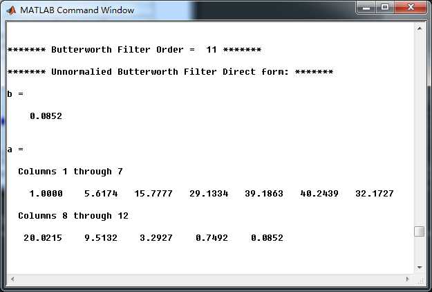
非归一化Butterworth模拟原型低通滤波器,直接形式的系数,
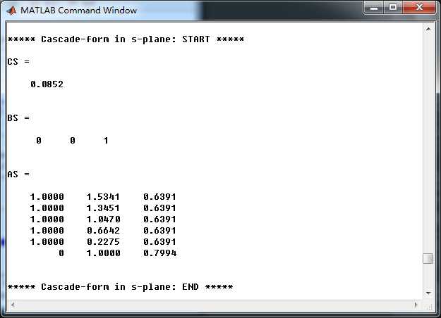
模拟低通串联形式的系数:
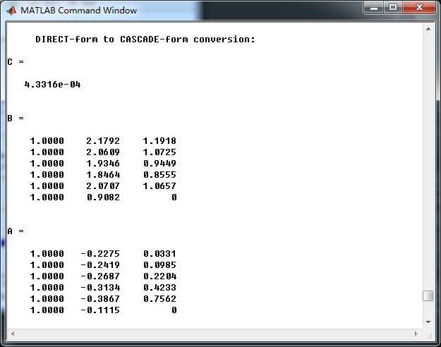
用双线性变换法,转换成数字Butterworth低通,直接形式的系数如下
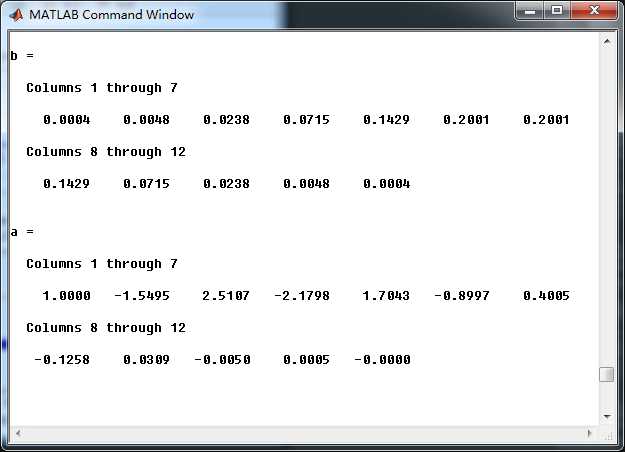
数字低通串联形式系数
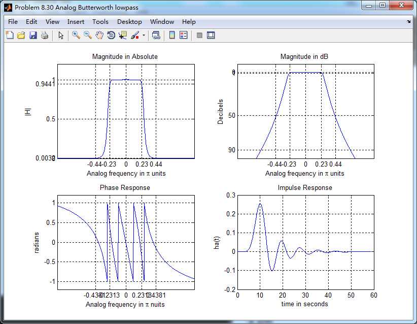
模拟Butterworth低通原型滤波器的幅度谱、相位谱和脉冲响应
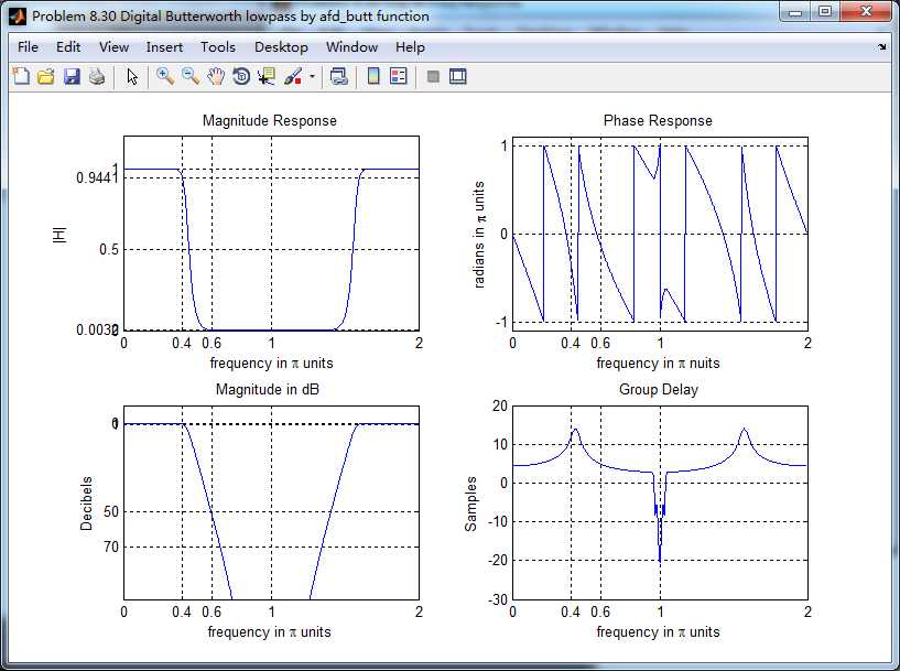
双线性变换法,得到的数字Butterworth低通滤波器,起幅度谱、相位谱和群延迟响应
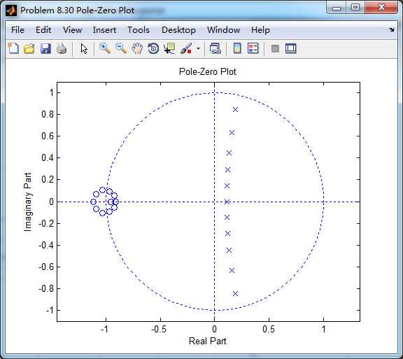
数字低通系统函数的零极点图
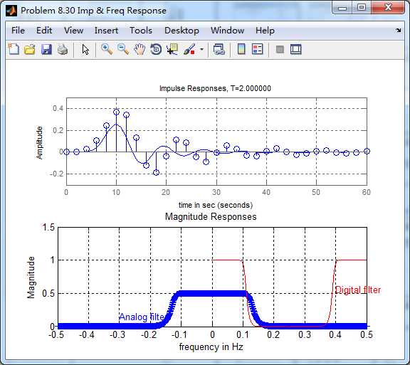
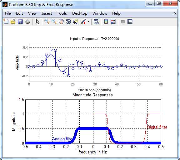
下图的上半部分,模拟低通和数字低通的脉冲响应对比,可以看出形态不一致。
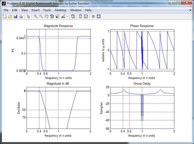
采用MATLAB自带的butter函数求取数字低通,其幅度谱、相位谱和群延迟。
与上面afd_butt函数所得结果相比,相位谱和群延迟稍有不同。
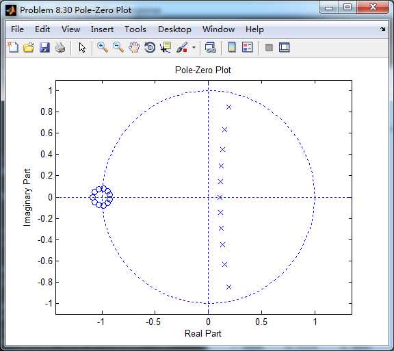
零极点图,也稍有不同,零点部分靠的更紧密。
脉冲响应,看不出区别。
《DSP using MATLAB》Problem 8.30
标签:title 模拟 his inf for elm Plan lan img
原文地址:https://www.cnblogs.com/ky027wh-sx/p/11616244.html