标签:tla 函数 max UNC number sam ann enc design

代码:
function [wpLP, wsLP, alpha] = bp2lpfre(wpbp, wsbp)
% Band-edge frequency conversion from bandpass to lowpass digital filter
% -------------------------------------------------------------------------
% [wpLP, wsLP, alpha] = bp2lpfre(wpbp, wsbp)
%   wpLP = passband edge for the lowpass digital prototype
%   wsLP = stopband edge for the lowpass digital prototype
%  alpha = lowpass to bandpass transformation parameter
%   wpbp = passband edge frequency array [wp_lower, wp_upper] for the bandpass
%   wshp = stopband edge frequency array [ws_lower, ws_upper] for the bandpass
%
%

% Determine the digital lowpass cutoff frequencies:
wpLP = 0.2*pi;
     K = cot((wpbp(2)-wpbp(1))/2)*tan(wpLP/2);
  beta = cos((wpbp(2)+wpbp(1))/2)/cos((wpbp(2)-wpbp(1))/2);
alpha1 = -2*beta*K/(K+1);
alpha2 = (K-1)/(K+1);

alpha = [alpha1, alpha2];

wsLP = -angle(-(exp(-2*j*wsbp(2))+alpha1*exp(-j*wsbp(2))+alpha2)/(alpha2*exp(-2*j*wsbp(2))+alpha1*exp(-j*wsbp(2))+1))
%wsLP = angle(-(exp(-2*j*wsbp(1))+alpha1*exp(-j*wsbp(1))+alpha2)/(alpha2*exp(-2*j*wsbp(1))+alpha1*exp(-j*wsbp(1))+1))
主程序代码:
%% ------------------------------------------------------------------------
%%            Output Info about this m-file
fprintf(‘\n***********************************************************\n‘);
fprintf(‘        <DSP using MATLAB> Problem 8.38.3 \n\n‘);

banner();
%% ------------------------------------------------------------------------

% Digital Filter Specifications:   Chebyshev-2 bandpass
wsbp = [0.30*pi 0.60*pi];             % digital stopband freq in rad
wpbp = [0.40*pi 0.50*pi];             % digital passband freq in rad
  Rp = 0.50;                          % passband ripple in dB
  As = 50;                            % stopband attenuation in dB

Ripple = 10 ^ (-Rp/20)           % passband ripple in absolute
Attn = 10 ^ (-As/20)             % stopband attenuation in absolute

fprintf(‘\n*******Digital bandpass, Coefficients of DIRECT-form***********\n‘);
[bbp, abp] = cheb2bpf(wpbp, wsbp, Rp, As);
[C, B, A] = dir2cas(bbp, abp)

% Calculation of Frequency Response:
[dbbp, magbp, phabp, grdbp, wwbp] = freqz_m(bbp, abp);

% ---------------------------------------------------------------
%    find Actual Passband Ripple and Min Stopband attenuation
% ---------------------------------------------------------------
delta_w = 2*pi/1000;
Rp_bp = -(min(dbbp(ceil(wpbp(1)/delta_w+1):1:ceil(wpbp(2)/delta_w+1))));      % Actual Passband Ripple

fprintf(‘\nActual Passband Ripple is %.4f dB.\n‘, Rp_bp);

As_bp = -round(max(dbbp(1:1:ceil(wsbp(1)/delta_w)+1)));                    % Min Stopband attenuation
fprintf(‘\nMin Stopband attenuation is %.4f dB.\n\n‘, As_bp);


%% -----------------------------------------------------------------
%%                             Plot
%% -----------------------------------------------------------------

figure(‘NumberTitle‘, ‘off‘, ‘Name‘, ‘Problem 8.38.3 Chebyshev-2 bp by cheb2bpf function‘)
set(gcf,‘Color‘,‘white‘);
M = 1;                          % Omega max

subplot(2,2,1); plot(wwbp/pi, magbp); axis([0, M, 0, 1.2]); grid on;
xlabel(‘Digital frequency in \pi units‘); ylabel(‘|H|‘); title(‘Magnitude Response‘);
set(gca, ‘XTickMode‘, ‘manual‘, ‘XTick‘, [0, 0.3, 0.4, 0.5, 0.6, M]);
set(gca, ‘YTickMode‘, ‘manual‘, ‘YTick‘, [0, 0.9441, 1]);

subplot(2,2,2); plot(wwbp/pi, dbbp); axis([0, M, -100, 2]); grid on;
xlabel(‘Digital frequency in \pi units‘); ylabel(‘Decibels‘); title(‘Magnitude in dB‘);
set(gca, ‘XTickMode‘, ‘manual‘, ‘XTick‘, [0, 0.3, 0.4, 0.5, 0.6, M]);
set(gca, ‘YTickMode‘, ‘manual‘, ‘YTick‘, [-80, -50, -1, 0]);
set(gca,‘YTickLabelMode‘,‘manual‘,‘YTickLabel‘,[‘80‘; ‘50‘;‘1 ‘;‘ 0‘]);


subplot(2,2,3); plot(wwbp/pi, phabp/pi); axis([0, M, -1.1, 1.1]); grid on;
xlabel(‘Digital frequency in \pi nuits‘); ylabel(‘radians in \pi units‘); title(‘Phase Response‘);
set(gca, ‘XTickMode‘, ‘manual‘, ‘XTick‘, [0, 0.3, 0.4, 0.5, 0.6, M]);
set(gca, ‘YTickMode‘, ‘manual‘, ‘YTick‘, [-1:0.5:1]);

subplot(2,2,4); plot(wwbp/pi, grdbp); axis([0, M, 0, 80]); grid on;
xlabel(‘Digital frequency in \pi units‘); ylabel(‘Samples‘); title(‘Group Delay‘);
set(gca, ‘XTickMode‘, ‘manual‘, ‘XTick‘, [0, 0.3, 0.4, 0.5, 0.6, M]);
set(gca, ‘YTickMode‘, ‘manual‘, ‘YTick‘, [0:20:80]);

figure(‘NumberTitle‘, ‘off‘, ‘Name‘, ‘Problem 8.38.3 Pole-Zero Plot‘)
set(gcf,‘Color‘,‘white‘);
zplane(bbp, abp);
title(sprintf(‘Pole-Zero Plot‘));
%pzplotz(b,a);


% -----------------------------------------------------
%              method 2  cheby2 function
% -----------------------------------------------------

% Calculation of Chebyshev-2 filter parameters:
[N, wn] = cheb2ord(wpbp/pi, wsbp/pi, Rp, As);

fprintf(‘\n  ********* Chebyshev-2 Filter Order is = %3.0f \n‘, N)

% Digital Chebyshev-2 Bandpass Filter Design:
[bbp, abp] = cheby2(N, As, wn);

[C, B, A] = dir2cas(bbp, abp)

% Calculation of Frequency Response:
[dbbp, magbp, phabp, grdbp, wwbp] = freqz_m(bbp, abp);

% ---------------------------------------------------------------
%    find Actual Passband Ripple and Min Stopband attenuation
% ---------------------------------------------------------------
delta_w = 2*pi/1000;
Rp_bp = -(min(dbbp(ceil(wpbp(1)/delta_w+1):1:ceil(wpbp(2)/delta_w+1))));      % Actual Passband Ripple

fprintf(‘\nActual Passband Ripple is %.4f dB.\n‘, Rp_bp);

As_bp = -round(max(dbbp(1:1:ceil(wsbp(1)/delta_w)+1)));                    % Min Stopband attenuation
fprintf(‘\nMin Stopband attenuation is %.4f dB.\n\n‘, As_bp);


%% -----------------------------------------------------------------
%%                             Plot
%% -----------------------------------------------------------------

figure(‘NumberTitle‘, ‘off‘, ‘Name‘, ‘Problem 8.38.3 Chebyshev-2 bp by cheby2 function‘)
set(gcf,‘Color‘,‘white‘);
M = 1;                          % Omega max

subplot(2,2,1); plot(wwbp/pi, magbp); axis([0, M, 0, 1.2]); grid on;
xlabel(‘Digital frequency in \pi units‘); ylabel(‘|H|‘); title(‘Magnitude Response‘);
set(gca, ‘XTickMode‘, ‘manual‘, ‘XTick‘, [0, 0.3, 0.4, 0.5, 0.6, M]);
set(gca, ‘YTickMode‘, ‘manual‘, ‘YTick‘, [0, 0.9441, 1]);

subplot(2,2,2); plot(wwbp/pi, dbbp); axis([0, M, -100, 2]); grid on;
xlabel(‘Digital frequency in \pi units‘); ylabel(‘Decibels‘); title(‘Magnitude in dB‘);
set(gca, ‘XTickMode‘, ‘manual‘, ‘XTick‘, [0, 0.3, 0.4, 0.5, 0.6, M]);
set(gca, ‘YTickMode‘, ‘manual‘, ‘YTick‘, [-80, -50, -1, 0]);
set(gca,‘YTickLabelMode‘,‘manual‘,‘YTickLabel‘,[‘80‘; ‘50‘;‘1 ‘;‘ 0‘]);


subplot(2,2,3); plot(wwbp/pi, phabp/pi); axis([0, M, -1.1, 1.1]); grid on;
xlabel(‘Digital frequency in \pi nuits‘); ylabel(‘radians in \pi units‘); title(‘Phase Response‘);
set(gca, ‘XTickMode‘, ‘manual‘, ‘XTick‘, [0, 0.3, 0.4, 0.5, 0.6, M]);
set(gca, ‘YTickMode‘, ‘manual‘, ‘YTick‘, [-1:0.5:1]);

subplot(2,2,4); plot(wwbp/pi, grdbp); axis([0, M, 0, 40]); grid on;
xlabel(‘Digital frequency in \pi units‘); ylabel(‘Samples‘); title(‘Group Delay‘);
set(gca, ‘XTickMode‘, ‘manual‘, ‘XTick‘, [0, 0.3, 0.4, 0.5, 0.6, M]);
set(gca, ‘YTickMode‘, ‘manual‘, ‘YTick‘, [0:10:40]);
运行结果:
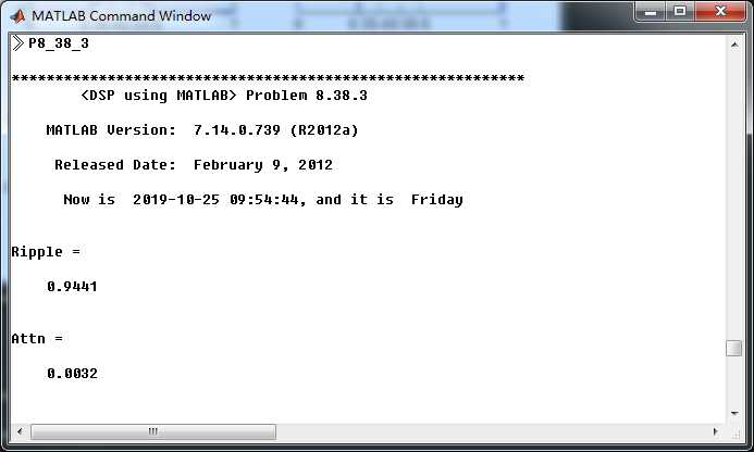
通带、阻带指标,绝对值单位,
采用cheb2bpf子函数,得到Chebyshev-2型数字带通滤波器,其系统函数串联形式的系数如下
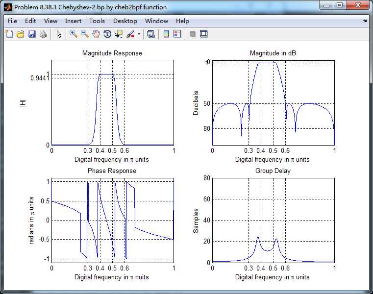
cheb2bpf函数得数字带通滤波器,幅度谱、相位谱和群延迟响应
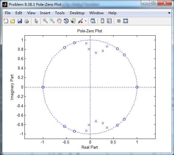
系统函数零极点图
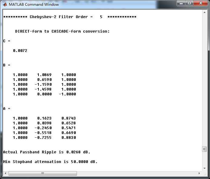
采用cheby2函数(MATLAB工具箱函数)得到Chebyshev-2型数字带通滤波器,其系统函数串联形式的系数如下,
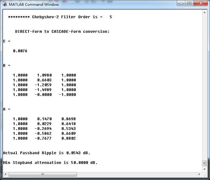
上图中的系数和cheb2bpf函数得到的系数相比,略有不同。
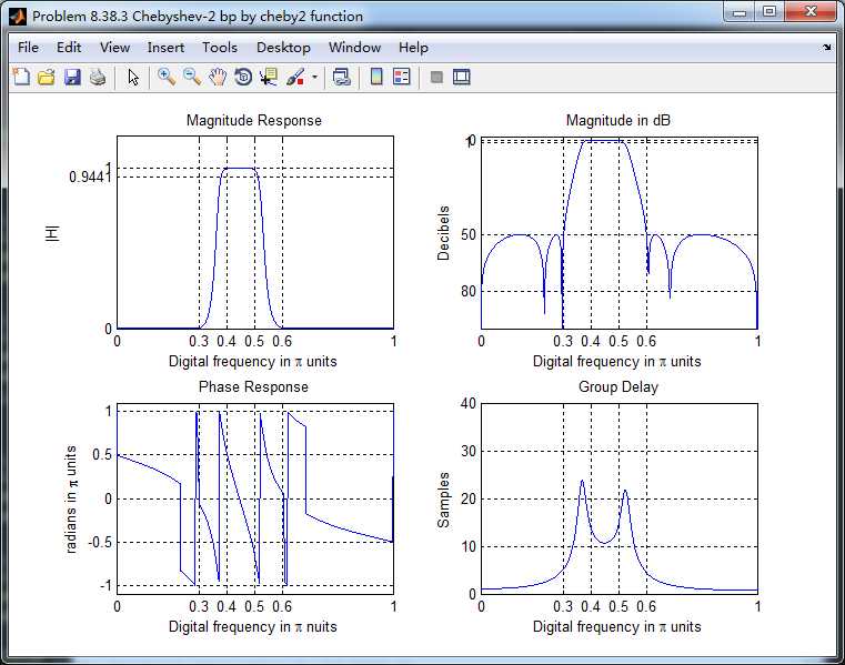
cheby2函数(MATLAB工具箱函数),得到的Chebyshev-2型数字带通滤波器,其幅度谱、相位谱和群延迟响应如下图
《DSP using MATLAB》Problem 8.38
标签:tla 函数 max UNC number sam ann enc design
原文地址:https://www.cnblogs.com/ky027wh-sx/p/11756171.html