标签:代码 code div eva alc http seq top 需要
代码:
%% ------------------------------------------------------------------------
%% Output Info about this m-file
fprintf(‘\n***********************************************************\n‘);
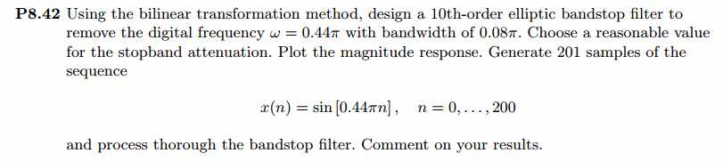
fprintf(‘ <DSP using MATLAB> Problem 8.42 \n\n‘);
banner();
%% ------------------------------------------------------------------------
% Digital Filter Specifications: Elliptic bandstop
wsbs = [0.40*pi 0.48*pi]; % digital stopband freq in rad
wpbs = [0.25*pi 0.75*pi]; % digital passband freq in rad
Rp = 1.0 % passband ripple in dB
As = 80 % stopband attenuation in dB
Ripple = 10 ^ (-Rp/20) % passband ripple in absolute
Attn = 10 ^ (-As/20) % stopband attenuation in absolute
% Calculation of Elliptic filter parameters:
[N, wn] = ellipord(wpbs/pi, wsbs/pi, Rp, As);
fprintf(‘\n ********* Elliptic Filter Order is = %3.0f \n‘, N)
% Digital Elliptic bandstop Filter Design:
[bbs, abs] = ellip(N, Rp, As, wn, ‘stop‘);
[C, B, A] = dir2cas(bbs, abs)
% Calculation of Frequency Response:
[dbbs, magbs, phabs, grdbs, wwbs] = freqz_m(bbs, abs);
% ---------------------------------------------------------------
% find Actual Passband Ripple and Min Stopband attenuation
% ---------------------------------------------------------------
delta_w = 2*pi/1000;
Rp_bs = -(min(dbbs(1:1:ceil(wpbs(1)/delta_w+1)))); % Actual Passband Ripple
fprintf(‘\nActual Passband Ripple is %.4f dB.\n‘, Rp_bs);
As_bs = -round(max(dbbs(ceil(wsbs(1)/delta_w)+1:1:ceil(wsbs(2)/delta_w)+1))); % Min Stopband attenuation
fprintf(‘\nMin Stopband attenuation is %.4f dB.\n\n‘, As_bs);
%% -----------------------------------------------------------------
%% Plot
%% -----------------------------------------------------------------
figure(‘NumberTitle‘, ‘off‘, ‘Name‘, ‘Problem 8.42 Elliptic bs by ellip function‘)
set(gcf,‘Color‘,‘white‘);
M = 1; % Omega max
subplot(2,2,1); plot(wwbs/pi, magbs); axis([0, M, 0, 1.2]); grid on;
xlabel(‘Digital frequency in \pi units‘); ylabel(‘|H|‘); title(‘Magnitude Response‘);
set(gca, ‘XTickMode‘, ‘manual‘, ‘XTick‘, [0, 0.25, 0.40, 0.48, 0.75, M]);
set(gca, ‘YTickMode‘, ‘manual‘, ‘YTick‘, [0, 0.01, 0.8913, 1]);
subplot(2,2,2); plot(wwbs/pi, dbbs); axis([0, M, -120, 2]); grid on;
xlabel(‘Digital frequency in \pi units‘); ylabel(‘Decibels‘); title(‘Magnitude in dB‘);
set(gca, ‘XTickMode‘, ‘manual‘, ‘XTick‘, [0, 0.25, 0.40, 0.48, 0.75, M]);
set(gca, ‘YTickMode‘, ‘manual‘, ‘YTick‘, [ -80, -40, 0]);
set(gca,‘YTickLabelMode‘,‘manual‘,‘YTickLabel‘,[‘80‘; ‘40‘;‘ 0‘]);
subplot(2,2,3); plot(wwbs/pi, phabs/pi); axis([0, M, -1.1, 1.1]); grid on;
xlabel(‘Digital frequency in \pi nuits‘); ylabel(‘radians in \pi units‘); title(‘Phase Response‘);
set(gca, ‘XTickMode‘, ‘manual‘, ‘XTick‘, [0, 0.25, 0.40, 0.48, 0.75, M]);
set(gca, ‘YTickMode‘, ‘manual‘, ‘YTick‘, [-1:0.5:1]);
subplot(2,2,4); plot(wwbs/pi, grdbs); axis([0, M, 0, 50]); grid on;
xlabel(‘Digital frequency in \pi units‘); ylabel(‘Samples‘); title(‘Group Delay‘);
set(gca, ‘XTickMode‘, ‘manual‘, ‘XTick‘, [0, 0.25, 0.40, 0.48, 0.75, M]);
set(gca, ‘YTickMode‘, ‘manual‘, ‘YTick‘, [0:20:50]);
% ------------------------------------------------------------
% PART 2
% ------------------------------------------------------------
% Discrete time signal
Ts = 1; % sample intevals
n1_start = 0; n1_end = 200;
n1 = [n1_start:n1_end]; % [0:200]
xn1 = sin(0.44*pi*n1); % digital signal
% ----------------------------
% DTFT of xn1
% ----------------------------
M = 500;
[X1, w] = dtft1(xn1, n1, M);
%magX1 = abs(X1);
angX1 = angle(X1); realX1 = real(X1); imagX1 = imag(X1);
magX1 = sqrt(realX1.^2 + imagX1.^2);
%% --------------------------------------------------------------------
%% START X(w)‘s mag ang real imag
%% --------------------------------------------------------------------
figure(‘NumberTitle‘, ‘off‘, ‘Name‘, ‘Problem 8.42 X1 DTFT‘);
set(gcf,‘Color‘,‘white‘);
subplot(2,1,1); plot(w/pi,magX1); grid on; %axis([-1,1,0,1.05]);
title(‘Magnitude Response‘);
xlabel(‘digital frequency in \pi units‘); ylabel(‘Magnitude |H|‘);
set(gca, ‘XTickMode‘, ‘manual‘, ‘XTick‘, [0, 0.2, 0.44, 0.6, 0.8, 1.0, 1.2, 1.4, 1.56, 1.8, 2]);
subplot(2,1,2); plot(w/pi, angX1/pi); grid on; %axis([-1,1,-1.05,1.05]);
title(‘Phase Response‘);
xlabel(‘digital frequency in \pi units‘); ylabel(‘Radians/\pi‘);
figure(‘NumberTitle‘, ‘off‘, ‘Name‘, ‘Problem 8.42 X1 DTFT‘);
set(gcf,‘Color‘,‘white‘);
subplot(2,1,1); plot(w/pi, realX1); grid on;
title(‘Real Part‘);
xlabel(‘digital frequency in \pi units‘); ylabel(‘Real‘);
set(gca, ‘XTickMode‘, ‘manual‘, ‘XTick‘, [0, 0.2, 0.44, 0.6, 0.8, 1.0, 1.2, 1.4, 1.56, 1.8, 2]);
subplot(2,1,2); plot(w/pi, imagX1); grid on;
title(‘Imaginary Part‘);
xlabel(‘digital frequency in \pi units‘); ylabel(‘Imaginary‘);
%% -------------------------------------------------------------------
%% END X‘s mag ang real imag
%% -------------------------------------------------------------------
% ------------------------------------------------------------
% PART 3
% ------------------------------------------------------------
yn1 = filter(bbs, abs, xn1);
n2 = n1;
% ----------------------------
% DTFT of yn1
% ----------------------------
M = 500;
[Y1, w] = dtft1(yn1, n2, M);
%magY1 = abs(Y1);
angY1 = angle(Y1); realY1 = real(Y1); imagY1 = imag(Y1);
magY1 = sqrt(realY1.^2 + imagY1.^2);
%% --------------------------------------------------------------------
%% START Y1(w)‘s mag ang real imag
%% --------------------------------------------------------------------
figure(‘NumberTitle‘, ‘off‘, ‘Name‘, ‘Problem 8.42 Y1 DTFT‘);
set(gcf,‘Color‘,‘white‘);
subplot(2,1,1); plot(w/pi,magY1); grid on; %axis([-1,1,0,1.05]);
title(‘Magnitude Response‘);
xlabel(‘digital frequency in \pi units‘); ylabel(‘Magnitude |H|‘);
subplot(2,1,2); plot(w/pi, angY1/pi); grid on; %axis([-1,1,-1.05,1.05]);
title(‘Phase Response‘);
xlabel(‘digital frequency in \pi units‘); ylabel(‘Radians/\pi‘);
figure(‘NumberTitle‘, ‘off‘, ‘Name‘, ‘Problem 8.42 Y1 DTFT‘);
set(gcf,‘Color‘,‘white‘);
subplot(2,1,1); plot(w/pi, realY1); grid on;
title(‘Real Part‘);
xlabel(‘digital frequency in \pi units‘); ylabel(‘Real‘);
subplot(2,1,2); plot(w/pi, imagY1); grid on;
title(‘Imaginary Part‘);
xlabel(‘digital frequency in \pi units‘); ylabel(‘Imaginary‘);
%% -------------------------------------------------------------------
%% END Y1‘s mag ang real imag
%% -------------------------------------------------------------------
figure(‘NumberTitle‘, ‘off‘, ‘Name‘, ‘Problem 8.42 x(n) and y(n)‘)
set(gcf,‘Color‘,‘white‘);
subplot(2,1,1); stem(n1, xn1);
xlabel(‘n‘); ylabel(‘x(n)‘);
title(‘xn sequence‘); grid on;
subplot(2,1,2); stem(n1, yn1);
xlabel(‘n‘); ylabel(‘y(n)‘);
title(‘yn sequence‘); grid on;
运行结果:
我自己假设通带1dB,阻带衰减80dB。
在此基础上设计指标,绝对单位,
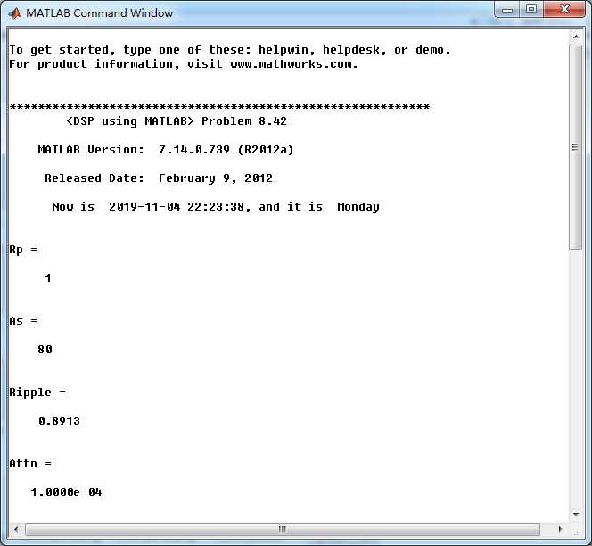
ellip函数(MATLAB工具箱函数)得到Elliptic带阻滤波器,阶数为5,系统函数串联形式系数如下图。
要想得到题目中的10阶的话,阻带衰减估计需要达到160dB左右,觉得没必要那么大。
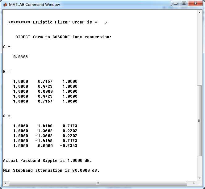
Elliptic带阻滤波器,幅度谱、相位谱和群延迟响应
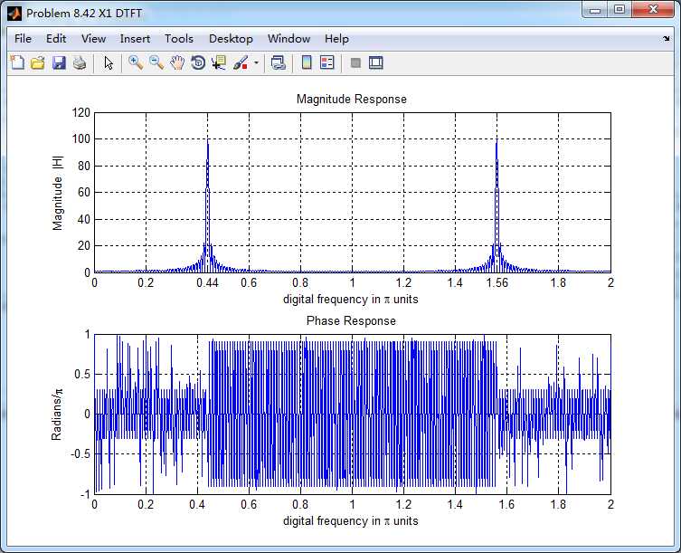
输入离散时间信号x(n)的谱如下,可看出,频率分量0.44π
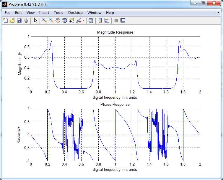
通过带阻滤波器后,得到的输出y(n)的谱,好像变乱了,o(╥﹏╥)o
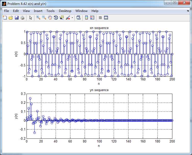
输入和输出的离散时间序列如下图
《DSP using MATLAB》Problem 8.42
标签:代码 code div eva alc http seq top 需要
原文地址:https://www.cnblogs.com/ky027wh-sx/p/11808896.html