标签:his 颜色 original 精确 大致 dsp seq nsa 抽取
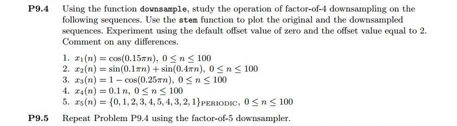
只放第1小题。
代码:
%% ------------------------------------------------------------------------
%% Output Info about this m-file
fprintf(‘\n***********************************************************\n‘);
fprintf(‘ <DSP using MATLAB> Problem 9.4.1 \n\n‘);
banner();
%% ------------------------------------------------------------------------
% ------------------------------------------------------------
% PART 1
% ------------------------------------------------------------
% Discrete time signal
n1_start = 0; n1_end = 100;
n1 = [n1_start:1:n1_end];
xn1 = cos(0.15*pi*n1); % digital signal
D = 4; % downsample by factor D
OFFSET = 0;
y = downsample(xn1, D, OFFSET);
ny = [n1_start:n1_end/D];
% ny = [n1_start:n1_end/D-1]; % OFFSET=2
figure(‘NumberTitle‘, ‘off‘, ‘Name‘, ‘Problem 9.4.1 xn1 and y‘)
set(gcf,‘Color‘,‘white‘);
subplot(2,1,1); stem(n1, xn1, ‘b‘);
xlabel(‘n‘); ylabel(‘x(n)‘);
title(‘xn1 original sequence‘); grid on;
subplot(2,1,2); stem(ny, y, ‘r‘);
xlabel(‘ny‘); ylabel(‘y(n)‘);
title(sprintf(‘y sequence, downsample by D=%d offset=%d‘, D, OFFSET)); grid on;
% ----------------------------
% DTFT of xn1
% ----------------------------
M = 500;
[X1, w] = dtft1(xn1, n1, M);
magX1 = abs(X1); angX1 = angle(X1); realX1 = real(X1); imagX1 = imag(X1);
max(magX1)
%% --------------------------------------------------------------------
%% START X(w)‘s mag ang real imag
%% --------------------------------------------------------------------
figure(‘NumberTitle‘, ‘off‘, ‘Name‘, ‘Problem 9.4.1 X1 DTFT‘);
set(gcf,‘Color‘,‘white‘);
subplot(2,1,1); plot(w/pi,magX1); grid on; %axis([-2, -1, -0.5, 0, 0.15, 0.5, 1, 2]);
title(‘Magnitude Response‘);
xlabel(‘digital frequency in \pi units‘); ylabel(‘Magnitude |H|‘);
set(gca, ‘xtick‘, [-2,-1.85,-1.5,-1,-0.15,0,0.15,0.5,1,1.5,1.85,2]);
subplot(2,1,2); plot(w/pi, angX1/pi); grid on; %axis([-1,1,-1.05,1.05]);
title(‘Phase Response‘);
xlabel(‘digital frequency in \pi units‘); ylabel(‘Radians/\pi‘);
figure(‘NumberTitle‘, ‘off‘, ‘Name‘, ‘Problem 9.4.1 X1 DTFT‘);
set(gcf,‘Color‘,‘white‘);
subplot(2,1,1); plot(w/pi, realX1); grid on;
title(‘Real Part‘);
xlabel(‘digital frequency in \pi units‘); ylabel(‘Real‘);
subplot(2,1,2); plot(w/pi, imagX1); grid on;
title(‘Imaginary Part‘);
xlabel(‘digital frequency in \pi units‘); ylabel(‘Imaginary‘);
%% -------------------------------------------------------------------
%% END X‘s mag ang real imag
%% -------------------------------------------------------------------
% ----------------------------
% DTFT of y
% ----------------------------
M = 500;
[Y, w] = dtft1(y, ny, M);
magY_DTFT = abs(Y); angY_DTFT = angle(Y); realY_DTFT = real(Y); imagY_DTFT = imag(Y);
max(magY_DTFT)
ratio = max(magX1)/max(magY_DTFT)
%% --------------------------------------------------------------------
%% START Y(w)‘s mag ang real imag
%% --------------------------------------------------------------------
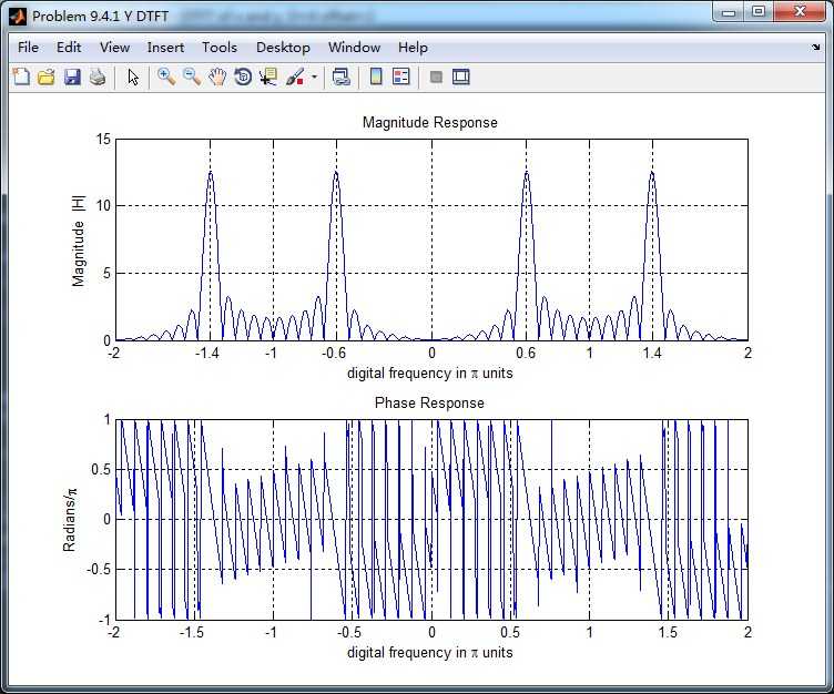
figure(‘NumberTitle‘, ‘off‘, ‘Name‘, ‘Problem 9.4.1 Y DTFT‘);
set(gcf,‘Color‘,‘white‘);
subplot(2,1,1); plot(w/pi, magY_DTFT); grid on; %axis([-2,2, -1, 2]);
title(‘Magnitude Response‘);
xlabel(‘digital frequency in \pi units‘); ylabel(‘Magnitude |H|‘);
set(gca, ‘xtick‘, [-2,-1.4,-1,-0.6,0,0.6,1,1.4,2]);
subplot(2,1,2); plot(w/pi, angY_DTFT/pi); grid on; %axis([-1,1,-1.05,1.05]);
title(‘Phase Response‘);
xlabel(‘digital frequency in \pi units‘); ylabel(‘Radians/\pi‘);
figure(‘NumberTitle‘, ‘off‘, ‘Name‘, ‘Problem 9.4.1 Y DTFT‘);
set(gcf,‘Color‘,‘white‘);
subplot(2,1,1); plot(w/pi, realY_DTFT); grid on;
title(‘Real Part‘);
xlabel(‘digital frequency in \pi units‘); ylabel(‘Real‘);
subplot(2,1,2); plot(w/pi, imagY_DTFT); grid on;
title(‘Imaginary Part‘);
xlabel(‘digital frequency in \pi units‘); ylabel(‘Imaginary‘);
%% -------------------------------------------------------------------
%% END Y‘s mag ang real imag
%% -------------------------------------------------------------------
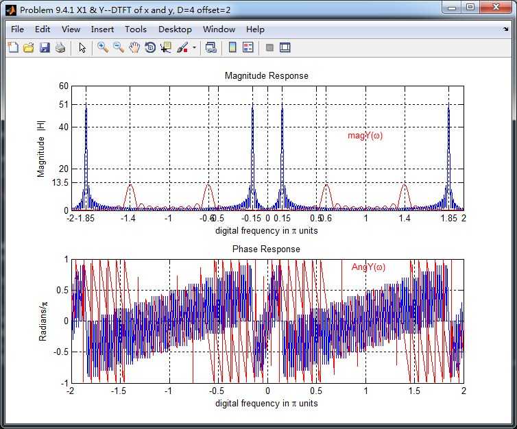
figure(‘NumberTitle‘, ‘off‘, ‘Name‘, sprintf(‘Problem 9.4.1 X1 & Y--DTFT of x and y, D=%d offset=%d‘, D,OFFSET));
set(gcf,‘Color‘,‘white‘);
subplot(2,1,1); plot(w/pi,magX1); grid on; %axis([-1,1,0,1.05]);
title(‘Magnitude Response‘);
xlabel(‘digital frequency in \pi units‘); ylabel(‘Magnitude |H|‘);
set(gca, ‘xtick‘, [-2,-1.85,-1.4,-1,-0.6,-0.5,-0.15,0,0.15,0.5,0.6,1,1.4,1.85,2]);
set(gca, ‘ytick‘, [-0.2, 0, 13.5, 20, 40, 51, 60]);
hold on;
plot(w/pi, magY_DTFT, ‘r‘); gtext(‘magY(\omega)‘, ‘Color‘, ‘r‘);
hold off;
subplot(2,1,2); plot(w/pi, angX1/pi); grid on; %axis([-1,1,-1.05,1.05]);
title(‘Phase Response‘);
xlabel(‘digital frequency in \pi units‘); ylabel(‘Radians/\pi‘);
hold on;
plot(w/pi, angY_DTFT/pi, ‘r‘); gtext(‘AngY(\omega)‘, ‘Color‘, ‘r‘);
hold off;
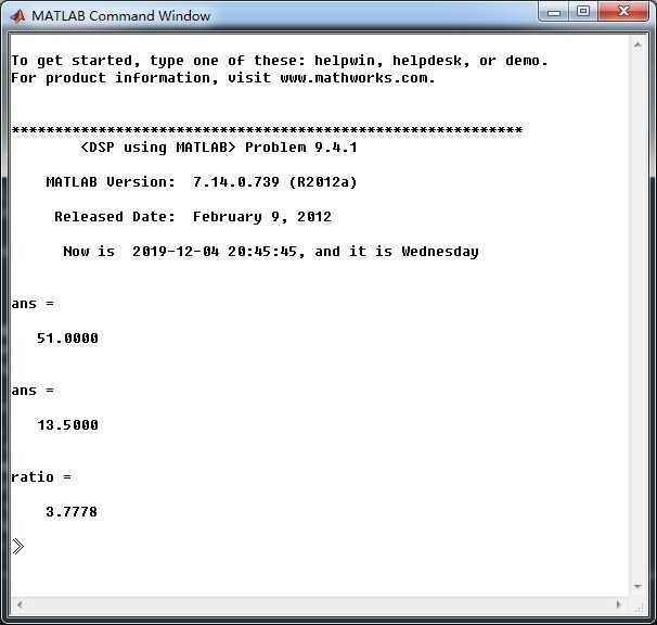
运行结果:
分两种情况
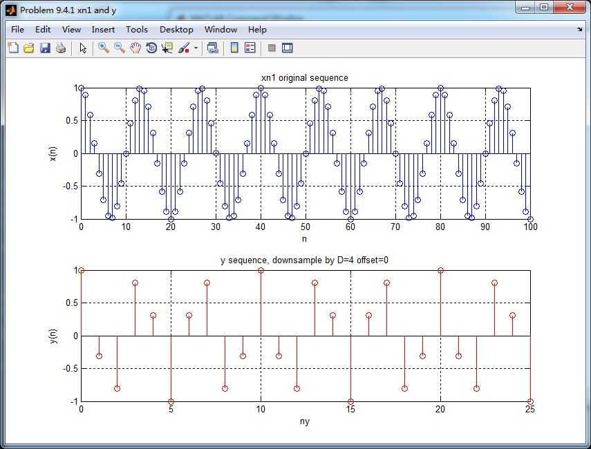
1、按照D=4抽取,offset=0
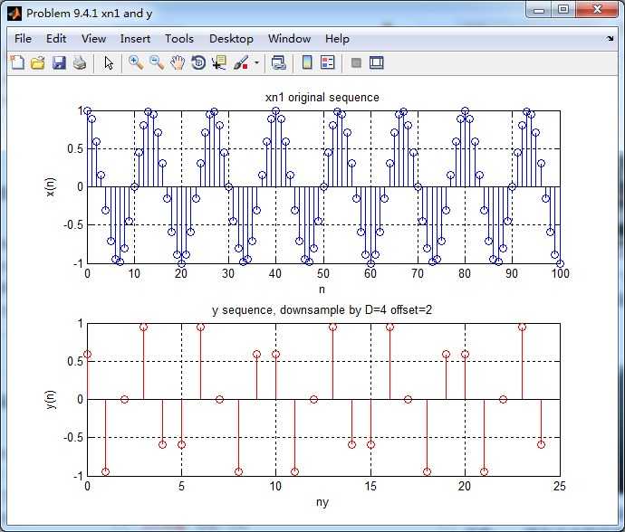
原始序列,抽取序列
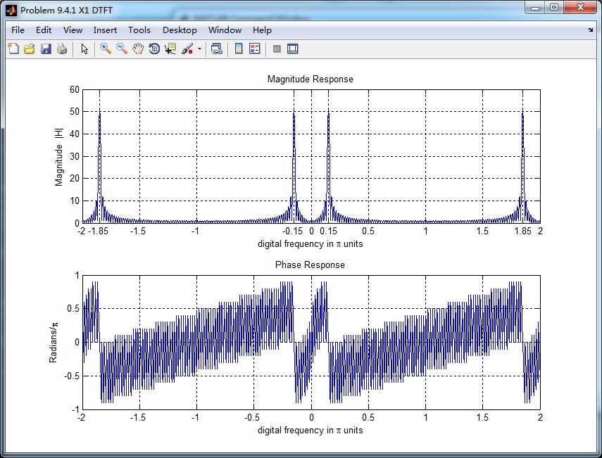
原始序列的谱
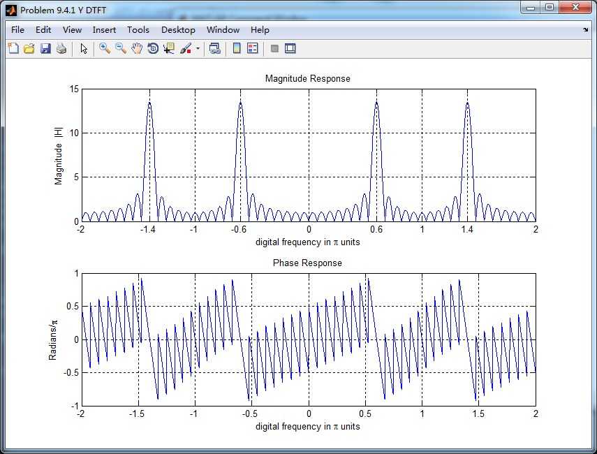
抽取序列的谱
二者的DTFT混叠到一起,红颜色曲线是抽取序列的DTFT,可看出,其幅度大致为原始序列的谱幅度的1/4(精确值是1/3.7778)。
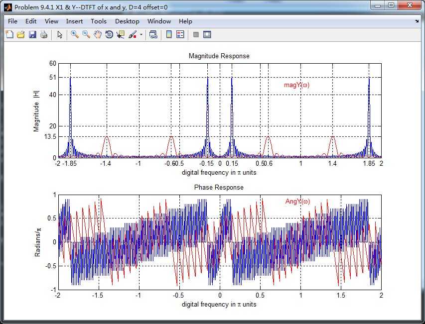
2、按照D=4抽取,offset=2
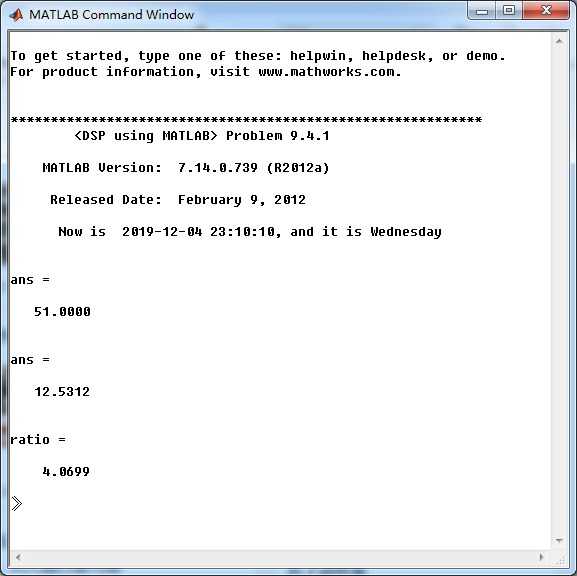
二者的DTFT混叠到一起,红颜色曲线是抽取序列的DTFT,可看出,其幅度大致为原始序列的谱幅度的1/4(精确值是1/4.0699)。
标签:his 颜色 original 精确 大致 dsp seq nsa 抽取
原文地址:https://www.cnblogs.com/ky027wh-sx/p/12003290.html