标签:define tac rsa speed column top elephant term city
为了代码更加可读,减少重复代码==lazy
You can type less code, saving effort and making your analyses more readable.
You can reuse your code from project to project.
查询函数的参数
> args(rank)
function (x, na.last = TRUE, ties.method = c("average", "first",
"last", "random", "max", "min")) 
# Update the function so heads have probability p_head
toss_coin <- function(n_flips,p_head) {
  coin_sides <- c("head", "tail")
  # Define a vector of weights
  weights <- c(p_head,1-p_head)
  # Modify the sampling to be weighted
  sample(coin_sides, n_flips, replace = TRUE,prob=weights)
}

# Generate 10 coin tosses
toss_coin(10,0.8)在定义函数的时候就已经赋值了
cut_by_quantile <- function(x, n=5, na.rm, labels, interval_type) {
  probs <- seq(0, 1, length.out = n + 1)
  qtiles <- quantile(x, probs, na.rm = na.rm, names = FALSE)
  right <- switch(interval_type, "(lo, hi]" = TRUE, "[lo, hi)" = FALSE)
  cut(x, qtiles, labels = labels, right = right, include.lowest = TRUE)
}

# Remove the n argument from the call
cut_by_quantile(
  n_visits,

  na.rm = FALSE,
  labels = c("very low", "low", "medium", "high", "very high"),
  interval_type = "(lo, hi]"
)
n是默认参数# Set the categories for interval_type to "(lo, hi]" and "[lo, hi)"
cut_by_quantile <- function(x, n = 5, na.rm = FALSE, labels = NULL,
interval_type = c("(lo, hi]", "[lo, hi)")) {
# Match the interval_type argument
interval_type <- match.arg(interval_type)
probs <- seq(0, 1, length.out = n + 1)
qtiles <- quantile(x, probs, na.rm = na.rm, names = FALSE)
right <- switch(interval_type, "(lo, hi]" = TRUE, "[lo, hi)" = FALSE)
cut(x, qtiles, labels = labels, right = right, include.lowest = TRUE)
}
# Remove the interval_type argument from the call
cut_by_quantile(n_visits)# From previous steps
get_reciprocal <- function(x) {
1 / x
}
calc_harmonic_mean <- function(x) {
x %>%
get_reciprocal() %>%
mean() %>%
get_reciprocal()
}
std_and_poor500 %>%
# Group by sector
group_by(sector) %>%
# Summarize, calculating harmonic mean of P/E ratio
summarize(hmean_pe_ratio = calc_harmonic_mean(pe_ratio))calc_harmonic_mean <- function(x, ...) {
x %>%
get_reciprocal() %>%
mean(...) %>%
get_reciprocal()
}
>
> std_and_poor500 %>%
# Group by sector
group_by(sector) %>%
# Summarize, calculating harmonic mean of P/E ratio
summarize(hmean_pe_ratio = calc_harmonic_mean(pe_ratio,na.rm=TRUE))
# A tibble: 11 x 2
sector hmean_pe_ratio
<chr> <dbl>
1 Communication Services 17.5
2 Consumer Discretionary 15.2
3 Consumer Staples 19.8
4 Energy 13.7
5 Financials 12.9
6 Health Care 26.6
7 Industrials 18.2
8 Information Technology 21.6
9 Materials 16.3
10 Real Estate 32.5
11 Utilities 23.9You can use the assert_*() functions from assertive to check inputs and throw errors when they fail.
calc_harmonic_mean <- function(x, na.rm = FALSE) {
  # Assert that x is numeric
  assert_is_numeric(x)
  x %>%
    get_reciprocal() %>%
    mean(na.rm = na.rm) %>%
    get_reciprocal()
}
弹出报错
calc_harmonic_mean <- function(x, na.rm = FALSE) {
  assert_is_numeric(x)
  # Check if any values of x are non-positive
  if(any(is_non_positive(x), na.rm = TRUE)) {
    # Throw an error
    stop("x contains non-positive values, so the harmonic mean makes no sense.")
  }
  x %>%
    get_reciprocal() %>%
    mean(na.rm = na.rm) %>%
    get_reciprocal()
}

# See what happens when you pass it negative numbers
calc_harmonic_mean(std_and_poor500$pe_ratio - 20)一直存在的且默认
Sometimes, you don‘t need to run through the whole body of a function to get the answer. In that case you can return early from that function using return().
To check if x is divisible by n, you can use is_divisible_by(x, n) from assertive.
Alternatively, use the modulo operator, %%. x %% n gives the remainder when dividing x by n, so x %% n == 0 determines whether x is divisible by n. Try 1:10 %% 3 == 0 in the console.
To solve this exercise, you need to know that a leap year is every 400th year (like the year 2000) or every 4th year that isn‘t a century (like 1904 but not 1900 or 1905).
is_leap_year <- function(year) {
  # If year is div. by 400 return TRUE
  if(is_divisible_by(year, 400)) {
    return(TRUE)
  }
  # If year is div. by 100 return FALSE
  if(is_divisible_by(year, 100)) {
    return(FALSE)
  }
  # If year is div. by 4 return TRUE
  if(is_divisible_by(year, 4)) {
    return(TRUE)
  }
  # Otherwise return FALSE
  FALSE
}
# Define a pipeable plot fn with data and formula args
pipeable_plot <- function(data, formula) {
# Call plot() with the formula interface
plot(formula, data)
# Invisibly return the input dataset
invisible(data)
}
# Draw the scatter plot of dist vs. speed again
plt_dist_vs_speed <- cars %>%
pipeable_plot(dist ~ speed)
# Now the plot object has a value
plt_dist_vs_speedGiven an R statistical model or other non-tidy object, add columns to the original dataset such as predictions, residuals and cluster assignments.
> # Use broom tools to get a list of 3 data frames
> list(
    # Get model-level values
    model = glance(model),
    # Get coefficient-level values
    coefficients = tidy(model),
    # Get observation-level values
    observations = augment(model)
  )
$model
# A tibble: 1 x 7
  null.deviance df.null logLik    AIC    BIC deviance df.residual
          <dbl>   <int>  <dbl>  <dbl>  <dbl>    <dbl>       <int>
1        18850.     345 -6425. 12864. 12891.   11529.         339

$coefficients
# A tibble: 7 x 5
  term              estimate std.error statistic   p.value
  <chr>                <dbl>     <dbl>     <dbl>     <dbl>
1 (Intercept)         4.09      0.0279   146.    0.
2 genderfemale        0.374     0.0212    17.6   2.18e- 69
3 income($25k,$55k]  -0.0199    0.0267    -0.746 4.56e-  1
4 income($55k,$95k]  -0.581     0.0343   -16.9   3.28e- 64
5 income($95k,$Inf)  -0.578     0.0310   -18.7   6.88e- 78
6 travel(0.25h,4h]   -0.627     0.0217   -28.8   5.40e-183
7 travel(4h,Infh)    -2.42      0.0492   -49.3   0.

$observations
# A tibble: 346 x 12
   .rownames n_visits gender income travel .fitted .se.fit  .resid    .hat
   <chr>        <dbl> <fct>  <fct>  <fct>    <dbl>   <dbl>   <dbl>   <dbl>
 1 25               2 female ($95k~ (4h,I~    1.46  0.0502  -1.24  0.0109
 2 26               1 female ($95k~ (4h,I~    1.46  0.0502  -1.92  0.0109
 3 27               1 male   ($95k~ (0.25~    2.88  0.0269  -5.28  0.0129
 4 29               1 male   ($95k~ (4h,I~    1.09  0.0490  -1.32  0.00711
 5 30               1 female ($55k~ (4h,I~    1.46  0.0531  -1.92  0.0121
 6 31               1 male   [$0,$~ [0h,0~    4.09  0.0279 -10.4   0.0465
 7 33              80 female [$0,$~ [0h,0~    4.46  0.0235  -0.710 0.0479
 8 34             104 female ($95k~ [0h,0~    3.88  0.0261   6.90  0.0332
 9 35              55 male   ($25k~ (0.25~    3.44  0.0222   3.85  0.0153
10 36             350 female ($25k~ [0h,0~    4.44  0.0206  21.5   0.0360
# ... with 336 more rows, and 3 more variables: .sigma <dbl>, .cooksd <dbl>,
#   .std.resid <dbl>
Magnificent multi-assignment! Returning many values is as easy as collecting them into a list. The groomed model has data frames that are easy to program against.
# From previous step
groom_model <- function(model) {
  list(
    model = glance(model),
    coefficients = tidy(model),
    observations = augment(model)
  )
}

# Call groom_model on model, assigning to 3 variables
c(mdl, cff, obs) %<-% groom_model(model)

# See these individual variables
mdl; cff; obs> # From previous step
> rsa_lst <- list(
capitals = capitals,
national_parks = national_parks,
population = population
)
>
> # Convert the list to an environment
> rsa_env <- list2env(rsa_lst )
>
> # List the structure of each variable
> ls.str(rsa_env)
capitals : Classes 'tbl_df', 'tbl' and 'data.frame': 3 obs. of 2 variables:
$ city : chr "Cape Town" "Bloemfontein" "Pretoria"
$ type_of_capital: chr "Legislative" "Judicial" "Administrative"
national_parks : chr [1:22] "Addo Elephant National Park" "Agulhas National Park" ...
population : Time-Series [1:5] from 1996 to 2016: 40583573 44819778 47390900 51770560 55908900> # From previous steps
> rsa_lst <- list(
capitals = capitals,
national_parks = national_parks,
population = population
)
> rsa_env <- list2env(rsa_lst)
>
> # Find the parent environment of rsa_env
> parent <- parent.env(rsa_env)
>
> # Print its name
> environmentName(parent )
[1] "R_GlobalEnv"查看是否定义了一个变量exists packages
> # Does population exist in rsa_env?
> exists("population", envir = rsa_env)
[1] TRUE
>
> # Does population exist in rsa_env, ignoring inheritance?
> exists("population", envir = rsa_env,inherits=FALSE)
[1] FALSE这里个人觉得编程语言是在某种程度上面是相通的,还是认真的学习好一门吧。不然最后都会放弃了,加油
# Write a function to convert sq. meters to hectares
sq_meters_to_hectares <- function(sq_meters) {
  sq_meters / 10000
}

# Write a function to convert acres to sq. yards
acres_to_sq_yards <- function(acres) {
  4840 * acres
}

# Write a function to convert acres to sq. yards
acres_to_sq_yards <- function(acres) {
  4840 * acres
}
常见农业单位换算
# Write a function to convert sq. yards to sq. meters
sq_yards_to_sq_meters <- function(sq_yards) {
  sq_yards %>%
    # Take the square root
    sqrt() %>%
    # Convert yards to meters
    yards_to_meters() %>%
    # Square it
    raise_to_power(2)
}# Load fns defined in previous steps
load_step3()
# Write a function to convert bushels to kg
bushels_to_kgs <- function(bushels, crop) {
bushels %>%
# Convert bushels to lbs for this crop
bushels_to_lbs(crop) %>%
# Convert lbs to kgs
lbs_to_kgs()
}# Wrap this code into a function
fortify_with_metric_units <- function(data, crop) {
data %>%
mutate(
farmed_area_ha = acres_to_hectares(farmed_area_acres),
yield_kg_per_ha = bushels_per_acre_to_kgs_per_hectare(
yield_bushels_per_acre,
crop = crop
)
)
}
# Try it on the wheat dataset
fortify_with_metric_units(wheat, crop = "wheat")绘图
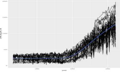
# Using corn, plot yield (kg/ha) vs. year
> ggplot(corn, aes(year, yield_kg_per_ha)) +
    # Add a line layer, grouped by state
    geom_line(aes(group = state)) +
    # Add a smooth trend layer
geom_smooth()# Wrap this code into a function
fortify_with_census_region<-function(data){
data %>%
inner_join(usa_census_regions, by = "state")
}
# Try it on the wheat dataset
fortify_with_census_region(wheat)# Wrap this code into a function
plot_yield_vs_year_by_region<-function(data){
plot_yield_vs_year(data) +
facet_wrap(vars(census_region))
}
# Try it on the wheat dataset
plot_yield_vs_year_by_region(wheat)
# Wrap the model code into a function
run_gam_yield_vs_year_by_region<-function(data){
  gam(yield_kg_per_ha ~ s(year) + census_region, data = corn)
}

# Try it on the wheat dataset
run_gam_yield_vs_year_by_region(wheat)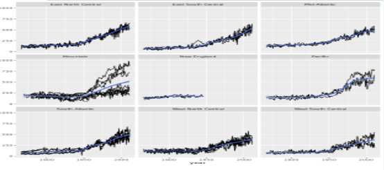
# Make predictions in 2050
predict_this <- data.frame(
  year = 2050,
  census_region = census_regions
)

# Predict the yield
pred_yield_kg_per_ha <- predict(corn_model, predict_this, type = "response")

predict_this %>%
  # Add the prediction as a column of predict_this
  mutate(pred_yield_kg_per_ha = pred_yield_kg_per_ha)
reference
Introduction to Writing Functions in R
标签:define tac rsa speed column top elephant term city
原文地址:https://www.cnblogs.com/gaowenxingxing/p/12068755.html