标签:数据分析 datetime 数据可视化 过程 diff get 夏天 title day
共享单车数据分析和共享单车用户行为分析PPT
从数据分析,到数据展示,完成一个完整数据分析项目的全部过程
共享单车由于其符合低碳出行理念,政府对这一新鲜事物也处于善意的观察期。

2017年12月,共享单车入选2017年民生热词榜。

2017年12月,ofo率先取消了免费月卡,月卡价格也已调整为20元/月。

2019年4月8日,哈罗单车宣布涨价,这是继小蓝单车、摩拜单车后第三家宣布涨价的共享单车。

2019年年底前,北京共享单车未接入监管平台将被视为违规投放。
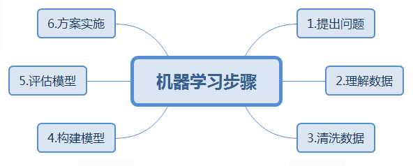
提出问题(Business Understanding )
理解数据(Data Understanding)
    采集数据
    导入数据
    查看数据集信息
数据清洗(Data Preparation )
    数据预处理
    特征工程(Feature Engineering)
构建模型(Modeling)
模型评估(Evaluation)
方案实施 (Deployment)
    提交结果到Kaggle
    报告撰写
影响骑车人数的因素有哪些?
3.1导入数据源
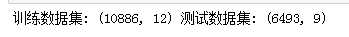
import warnings
warnings.filterwarnings(‘ignore‘)
#导入处理数据包
import numpy as np
import pandas as pd
#导入数据
#训练数据集
train = pd.read_csv("train_bike.csv")
#测试数据集
test  = pd.read_csv("test_bike.csv")
#这里要记住训练数据集有891条数据,方便后面从中拆分出测试数据集用于提交Kaggle结果
print (‘训练数据集:‘,train.shape,‘测试数据集:‘,test.shape)
3.2.查看各字段数据类型、缺失值
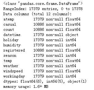
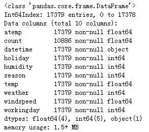
print(‘训练数据集:‘,train.info(),‘测试数据集:‘,test.info())
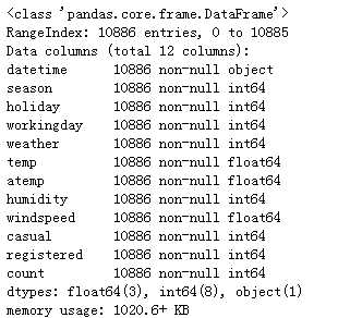
训练集和测试集没有缺失值
3.3 查看数据集信息
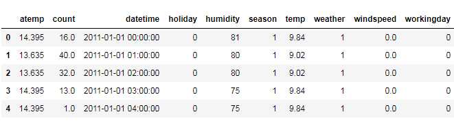
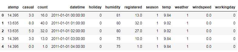
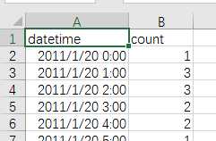
train.head()

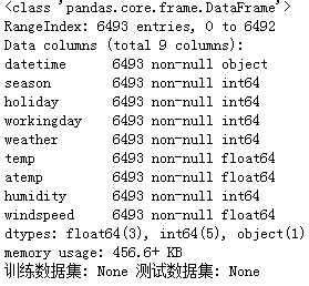
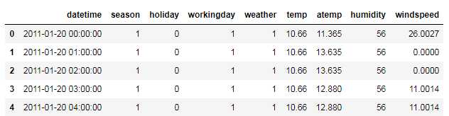
test.head()
数据说明:
分析:
1.训练数据集:

    总共10886行,12列,各字段均无缺失值

    除时间列数据为字符串外其余都为数值型数据:时间的数据格式需要转换为时间序列,进一步处理得到日期和星期的时间数据

    count=casual+registered,要探求影响租车量的因素,因而这两列可删去

2.测试数据集:

    总共6493行,9列,各字段均无缺失值
    测试数据集完整无需预处理


字段说明
Data Fields

    datetime时间 - 年月日小时
    season季节 - 1 = spring春天, 2 = summer夏天, 3 = fall秋天, 4 = winter冬天
    holiday节假日 - 0:否,1:是
    workingday工作日 - 该天既不是周末也不是假日(0:否,1:是)
    weather天气 - 1:晴天,2:阴天 ,3:小雨或小雪 ,4:恶劣天气(大雨、冰雹、暴风雨或者大雪)
    temp实际温度 - 摄氏度
    atemp体感温度 - 摄氏度
    humidity湿度 - 相对湿度
    windspeed风速 - 风速
    casual - 未注册用户租借数量
    registered - 注册用户租借数量
    count - 总租借数量
将训练集和测试集放一起处理
full =train.append(test,ignore_index=True)
full.head()
full.info()
选择子集、列表重命名本例不需要
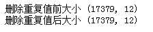
4.1删除重复值
print(‘删除重复值前大小‘,full.shape)

# 删除重复销售记录
full = full.drop_duplicates()

print(‘删除重复值后大小‘,full.shape)
合并后出现缺失值:主要是casual - 未注册用户租借数量、 registered - 注册用户租借数量
考虑到目前都是注册用户才能使用共享单车,我们删除casual和registered
4.2 处理缺失值
没有缺失值
#先备份测试数据集
bikeDf=full
我们删除casual和registered
bikeDf.drop(‘casual‘,axis=1,inplace=True)
bikeDf.drop(‘registered‘,axis=1,inplace=True)
bikeDf.head()
bikeDf.info()
(count)这里一列是我们的标签,用来做机器学习预测的,不需要处理这一列
4.3 特征提取(一致化处理)
4.3.1数据分类
‘‘‘
1.数值类型:

    temp实际温度 - 摄氏度
    atemp体感温度 - 摄氏度
    humidity湿度 - 相对湿度
    windspeed风速 - 风速
    count - 总租借数量

2.时间序列:

   datetime时间 - 年月日小时

3.分类数据:
1)有直接类别的


    season季节 - 1 = spring春天, 2 = summer夏天, 3 = fall秋天, 4 = winter冬天
    holiday节假日 - 0:否,1:是
    workingday工作日 - 该天既不是周末也不是假日(0:否,1:是)
    weather天气 - 1:晴天,2:阴天 ,3:小雨或小雪 ,4:恶劣天气(大雨、冰雹、暴风雨或者大雪)


2)字符串类型:可能从这里面提取出特征来,也归到分类数据中
onehot编码的优点可以总结如下:
1、能够处理非连续型数值特征。

2、在一定程度上也扩充了特征。比如性别本身是一个特征,经过one hot编码以后,就变成了男或女两个特征。
对于sex这样 处理后 只两个的特征的 暂时不作 onehot编码处理
4.3.2 数值类型数据不用处理
4.3.3 处理时间序列
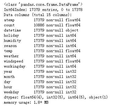
from datetime import datetime
#1、日月年拆解
bikeDf[‘year‘]=bikeDf[‘datetime‘].map(lambda s:s.split(‘-‘)[0]).astype(‘int‘)
bikeDf[‘month‘]=bikeDf[‘datetime‘].map(lambda s:s.split(‘-‘)[1]).astype(‘int‘)
bikeDf[‘day‘]=bikeDf[‘datetime‘].map(lambda s:s.split(‘-‘)[2].split()[0]).astype(‘int‘)
bikeDf[‘hour‘]=bikeDf[‘datetime‘].map(lambda s:s.split()[1].split(‘:‘)[0]).astype(‘int‘)
bikeDf[‘weekday‘]=bikeDf[‘datetime‘].map(lambda s:datetime.strptime(s.split()[0],‘%Y-%m-%d‘).weekday()).astype(‘int‘)
bikeDf.info()
4.3.4 处理分类数据
我们这里只处理:季节和天气
bikeDf[‘season‘].head()
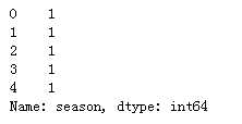
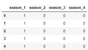
#存放提取后的特征
seasonDf = pd.DataFrame()
print(seasonDf )

‘‘‘
使用get_dummies进行one-hot编码,产生虚拟变量(dummy variables),列名前缀是prefix=Embarked
‘‘‘
seasonDf = pd.get_dummies( bikeDf[‘season‘] , prefix=‘season‘ )
seasonDf.head()
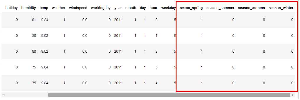
seasonDf .rename(columns={‘season_1‘:‘seaon_spring‘,‘season_2‘:‘season_summer‘,‘season_3‘:‘season_autumn‘,‘season_4‘:‘season_winter‘},inplace=True)
seasonDf.head()

#添加one-hot编码产生的虚拟变量(dummy variables)到数据集 bikeDf

bikeDf = pd.concat([bikeDf,seasonDf],axis=1)

‘‘‘


所以这里把season删掉
‘‘‘
bikeDf.drop(‘season‘,axis=1,inplace=True)
bikeDf.head()
天气
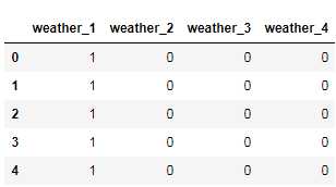
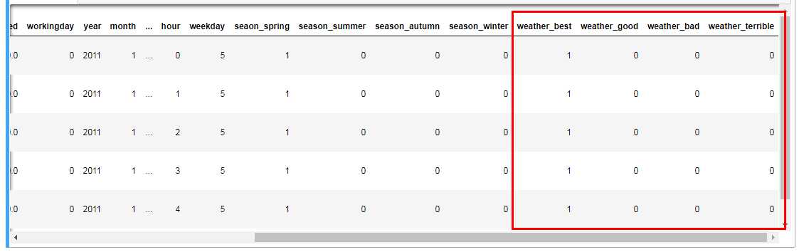
#存放提取后的特征
weatherDf = pd.DataFrame()
print(weatherDf)

‘‘‘
使用get_dummies进行one-hot编码,产生虚拟变量(dummy variables),列名前缀是prefix=Embarked
‘‘‘
weatherDf = pd.get_dummies( bikeDf[‘weather‘] , prefix=‘weather‘ )
weatherDf.head()
weatherDf.rename(columns={‘weather_1‘:‘weather_best‘,‘weather_2‘:‘weather_good‘,‘weather_3‘:‘weather_bad‘,‘weather_4‘:‘weather_terrible‘},inplace=True)
#添加one-hot编码产生的虚拟变量(dummy variables)到数据集 bikeDf

bikeDf = pd.concat([bikeDf,weatherDf],axis=1)

‘‘‘


所以这里把season删掉
‘‘‘
bikeDf.drop(‘weather‘,axis=1,inplace=True)
bikeDf.head()
4.4异常值处理
bikeDf.describe()
#描述指标:查看出“”值不能小于0
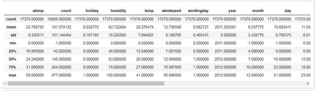
无异常值
5.1 特征选择
相关系数法:计算各个特征的相关系数
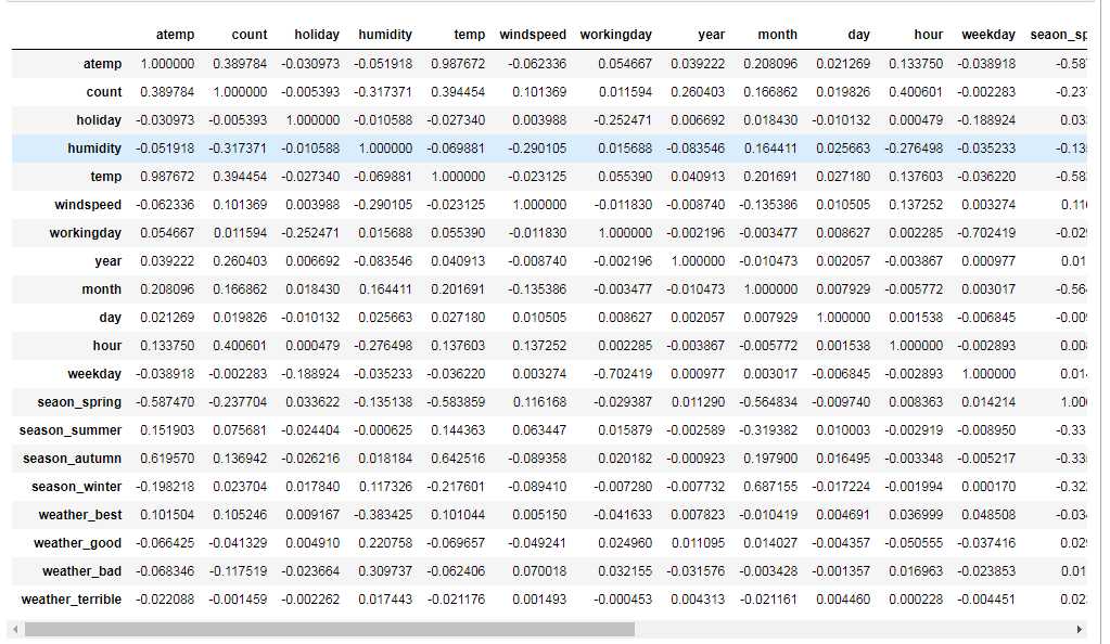
#相关性矩阵
corrDf = bikeDf.corr()
corrDf
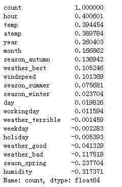
‘‘‘
查看各个特征与生成情况(Survived)的相关系数,
ascending=False表示按降序排列

‘‘‘
corrDf[‘count‘].sort_values(ascending =False)
特征值选择
根据各个特征与(count)的相关系数大小,我们选择了这几个特征作为模型的输入:
hour
temp
atemp
year
month
seasonDf
weatherDf
humidity
windspeed
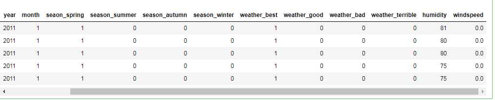
#特征选择
full_X = pd.concat([bikeDf[‘hour‘],
                   bikeDf[‘temp‘],
                   bikeDf[‘atemp‘],
                   bikeDf[‘year‘],
                   bikeDf[‘month‘],
                   seasonDf,
                   weatherDf,
                   bikeDf[‘humidity‘],
                   bikeDf[‘windspeed‘],
                      ],axis=1 )
full_X.head()
6.1使用热力图分析特征值与
import matplotlib.pyplot as plt
import seaborn as sns

#数据相关系数的一半
mask = np.array(bikeDf_corr)
mask[np.tril_indices_from(mask)] = False
#建立画板
fig=plt.figure(figsize=(12,12))
#建立画纸
ax1=fig.add_subplot(1,1,1)
#使用heatmap
sns.heatmap(bikeDf_corr, mask=mask, ax=ax1,square=False,annot=True)


plt.show()
plt.savefig(‘hot_photo.png‘)
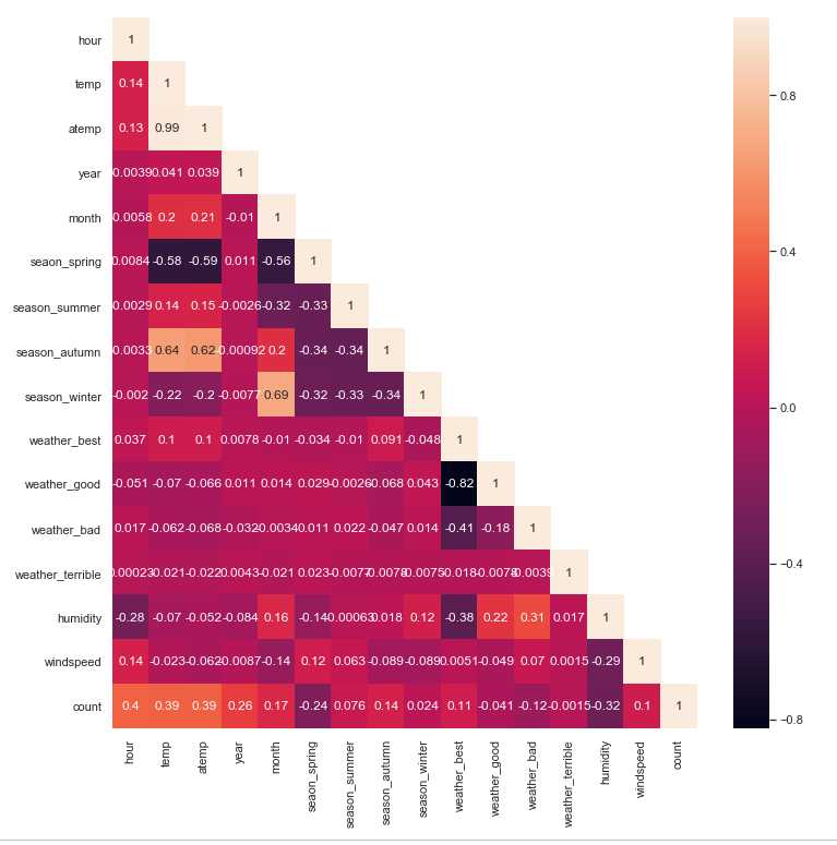
分析得出:
总租借数量(count)成正相关的有:
    hour
    temp(实际温度)
    atemp(体感温度)
    year
    month
    seasonDf
总租借数量(count)负相关的有:
    weatherDf
    humidity(湿度)
    windspeed(风速)
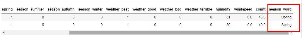
6.1租车人数在各特征值下的箱线图
# 季节变量离散化
full_X_1 = pd.concat([full_X,bikeDf[‘count‘]],axis=1)
seasonDict={1:‘Spring‘,2:‘Summer‘,3:‘autumn‘,4:‘Winter‘}
full_X_1[‘season_word‘]=full[‘season‘].map(seasonDict)
full_X_1.head(2)
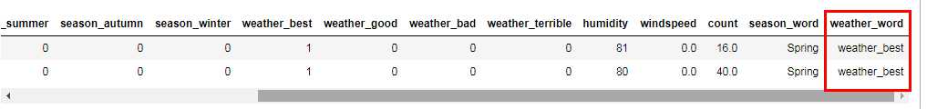
#天气变量离散化
weatherDict={1:‘weather_best‘,2:‘weather_good‘,3:‘weather_bad‘,4:‘weather_terrible‘}
full_X_1[‘weather_word‘]=full[‘weather‘].map(weatherDict)
full_X_1.head(2)
fig, axes = plt.subplots(3, 2)
fig.suptitle("ShareBike Analysis",fontsize=20,fontweight="bold")
sns.set(style=‘darkgrid‘)
fig.set_size_inches(15, 20)

ax1=sns.boxplot(data=full_X_1,y=‘count‘,orient=‘v‘,ax=axes[0][0])#count箱线图
ax2=sns.boxplot(data=full_X_1,x=‘hour‘,y=‘count‘,orient=‘v‘,ax=axes[0][1])

ax3=sns.boxplot(data=full_X_1,x=‘year‘,y=‘count‘,orient=‘v‘,ax=axes[1][0])
ax4=sns.boxplot(data=full_X_1,x=‘month‘,y=‘count‘,orient=‘v‘,ax=axes[1][1])
ax5=sns.boxplot(data=full_X_1,x=‘season_word‘,y=‘count‘,orient=‘v‘,ax=axes[2][0])
ax6=sns.boxplot(data=full_X_1,x=‘weather_word‘,y=‘count‘,orient=‘v‘,ax=axes[2][1])


axes[0][0].set(ylabel=‘Count‘,title="Box Plot On Count ")
axes[0][1].set(xlabel=‘hour‘, ylabel=‘Count‘,title="Box Plot On Count Across hour")

axes[1][0].set(xlabel=‘year‘, ylabel=‘Count‘,title="Box Plot On Count Across year")
axes[1][1].set(xlabel=‘month‘, ylabel=‘Count‘,title="Box Plot On Count Across month")
axes[2][0].set(xlabel=‘season_word‘, ylabel=‘Count‘,title="Box Plot On Count Across season_word")
axes[2][1].set(xlabel=‘weather_word‘, ylabel=‘Count‘,title="Box Plot On Count Across weather_word")

plt.savefig(‘subplots_photo1.png‘)
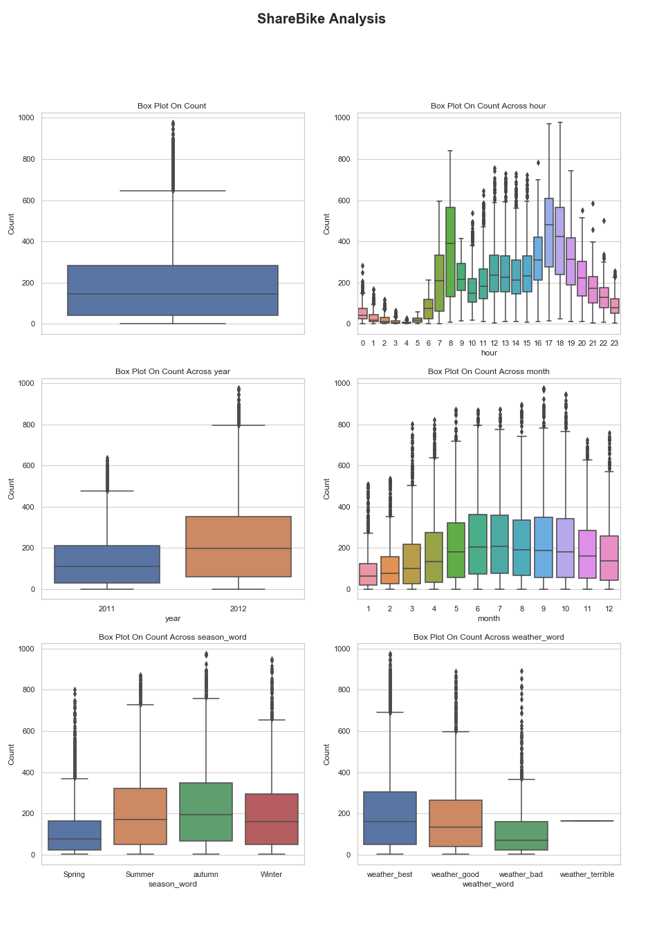
分析得出:
1、租车人数在150左右
2、一天中,出现两个用车高峰,一个是上午8点、一个是下午17点。分析原因可能是早晚高峰出行,导致用车人数增多。
3、秋季与夏季天气温暖租车量较高,春天最少
4、2012年相比2011年,租车人数中位数上升,共享单车出行方式市场越好
5、天气好时的用车中位数明显高于坏天气的中位数
# 由于
temp(实际温度)
atemp(体感温度)
humidity(湿度)
windspeed(风速)
参数较多,不方便用箱型图
6.2查看温度、体感温度、湿度与风速的分布情况
fig, axes = plt.subplots(2, 2)
fig.set_size_inches(12,10)

sns.distplot(full_X_1[‘temp‘],ax=axes[0,0])
sns.distplot(full_X_1[‘atemp‘],ax=axes[0,1])
sns.distplot(full_X_1[‘humidity‘],ax=axes[1,0])
sns.distplot(full_X_1[‘windspeed‘],ax=axes[1,1])

axes[0,0].set(xlabel=‘temp‘,title=‘Distribution of temp‘,)
axes[0,1].set(xlabel=‘atemp‘,title=‘Distribution of atemp‘)
axes[1,0].set(xlabel=‘humidity‘,title=‘Distribution of humidity‘)
axes[1,1].set(xlabel=‘windspeed‘,title=‘Distribution of windspeed‘)
plt.savefig(‘distplot_1.png‘)
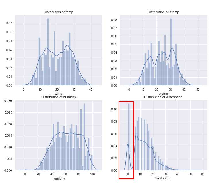
通过这个分布可以发现一些问题,比如风速为什么0的数据很多,而观察统计描述发现空缺值在1--6之间,

从这里似乎可以推测,数据本身或许是有缺失值的,但是用0来填充了,

但这些风速为0的数据会对预测产生干扰,希望使用随机森林根据相同的年份,月份,季节,温度,湿度等几个特征来填充一下风速的缺失值。

填充之前看一下非零数据的描述统计。
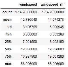
full_X_1[full_X_1["windspeed"]!=0]["windspeed"].describe()
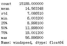
from sklearn.ensemble import RandomForestRegressor

full_X_1["windspeed_rfr"]=full_X_1["windspeed"]
# 将数据分成风速等于0和不等于两部分
dataWind0 = full_X_1[full_X_1["windspeed_rfr"]==0]
dataWindNot0 = full_X_1[full_X_1["windspeed_rfr"]!=0]
#选定模型
rfModel_wind = RandomForestRegressor(n_estimators=1000,random_state=42)
# 选定特征值

windColumns = [‘seaon_spring‘,‘season_summer‘,‘season_autumn‘,‘weather_best‘,‘weather_good‘,‘weather_bad‘,‘weather_terrible‘,‘season_winter‘,"humidity","month","temp","year","atemp"]
# 将风速不等于0的数据作为训练集,fit到RandomForestRegressor之中
rfModel_wind.fit(dataWindNot0[windColumns], dataWindNot0["windspeed_rfr"])
#通过训练好的模型预测风速
wind0Values = rfModel_wind.predict(X= dataWind0[windColumns])
#将预测的风速填充到风速为零的数据中
dataWind0.loc[:,"windspeed_rfr"] = wind0Values
#连接两部分数据
full_X_1 = dataWindNot0.append(dataWind0)
full_X_1.reset_index(inplace=True)
full_X_1.drop(‘index‘,inplace=True,axis=1)
fig, axes = plt.subplots(2, 2)
fig.set_size_inches(12,10)

sns.distplot(full_X_1[‘temp‘],ax=axes[0,0])
sns.distplot(full_X_1[‘atemp‘],ax=axes[0,1])
sns.distplot(full_X_1[‘humidity‘],ax=axes[1,0])
sns.distplot(full_X_1[‘windspeed_rfr‘],ax=axes[1,1])

axes[0,0].set(xlabel=‘temp‘,title=‘Distribution of temp‘,)
axes[0,1].set(xlabel=‘atemp‘,title=‘Distribution of atemp‘)
axes[1,0].set(xlabel=‘humidity‘,title=‘Distribution of humidity‘)
axes[1,1].set(xlabel=‘windspeed‘,title=‘Distribution of windspeed‘)
plt.savefig(‘distplot_2.png‘)
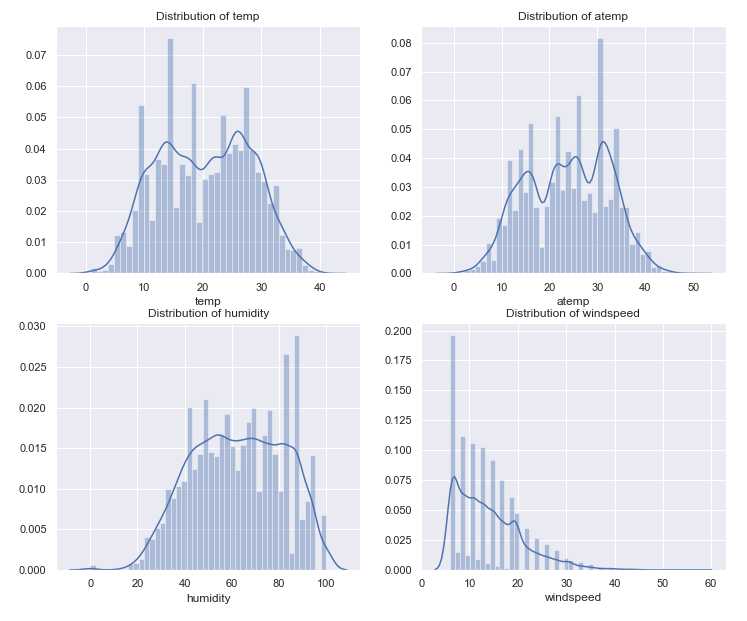
temp(实际温度) 主要分布在10到20
atemp(体感温度) 主要分布在20-30
humidity(湿度)主要分布在40-80
windspeed_rfr(风速)主要分布在5-10
full_X_1[[‘windspeed‘,‘windspeed_rfr‘]].describe()
可视化并观察数据
6.3整体观察
sns.pairplot(full_X_1 ,x_vars=[‘hour‘,‘year‘,‘month‘,‘season_word‘,‘weather_word‘,‘windspeed_rfr‘,‘humidity‘,‘temp‘,‘atemp‘] ,
             y_vars=[‘count‘] , plot_kws={‘alpha‘: 0.5})
plt.savefig(‘pairplot.png‘)
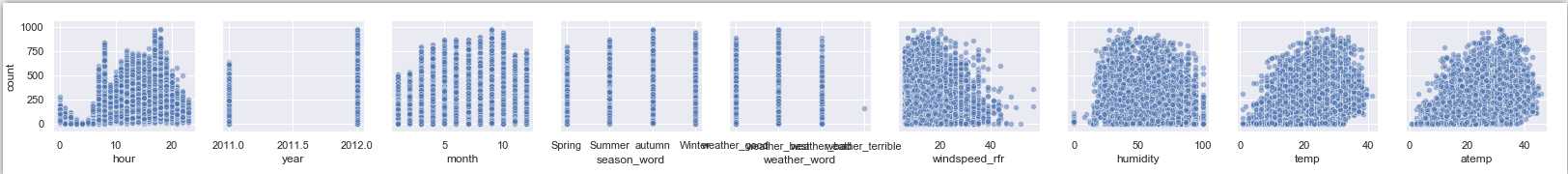
时间hour 出现两个峰值
时间year 租车数量逐年提升
月份month 租车数量集中在5-10月
季节season 租车重数在秋天
天气wheather 天气好坏直接影响租车数量
风速windspeed 与count成负相关
湿度humidity 租车数量集中在50
温度temp 租车数量集中在20-30
体表温度atemp 猪车数量集中在20-30
6.4逐项分析 折线图
6.4.1时间和count关系
#设置画框尺寸
fig = plt.figure(figsize=(18,6))
day_df = full_X_1.groupby([‘hour‘], as_index=True).agg({‘count‘:‘mean‘})
day_df.plot(figsize=(15,5),title = ‘The average number of rentals initiated per hour in the working day‘)
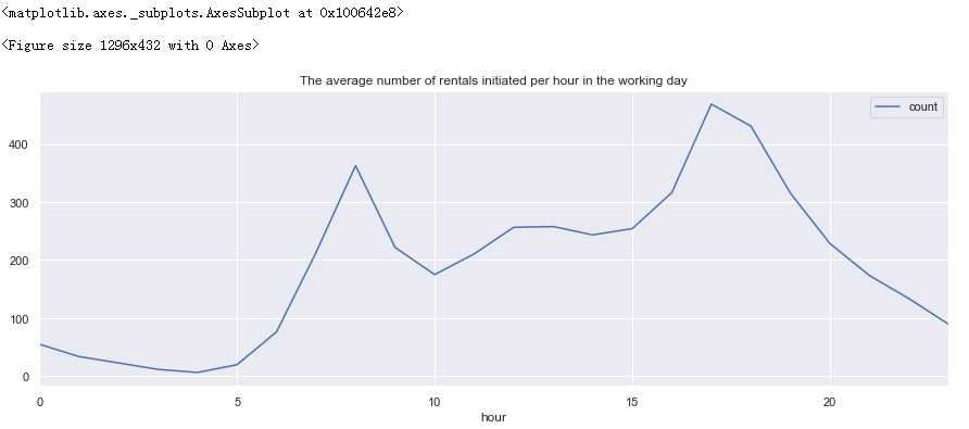
分析:
每天上下班时间是两个用车高峰,而中午也会有一个小高峰,猜测可能是外出午餐的人
6.4.2 温度对租赁数量的影响
先观察温度的走势
#设置画框尺寸
fig = plt.figure(figsize=(18,6))
day_df = full_X_1.groupby([‘month‘], as_index=True).agg({‘count‘:‘mean‘})
day_df.plot(figsize=(15,5),title = ‘The average number of rentals initiated per month‘)
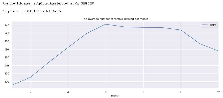
分析:
2-4月租车人数逐月提升
6-10达到峰值并趋于平缓
10月后租车人数出现下降
6.4.3 天气
#设置画框尺寸
fig = plt.figure(figsize=(18,6))
day_df = full_X_1.groupby([‘weather_word‘], as_index=True).agg({‘count‘:‘mean‘})
day_df.plot(figsize=(15,5),title = ‘The average number of rentals initiated per weather_word‘)
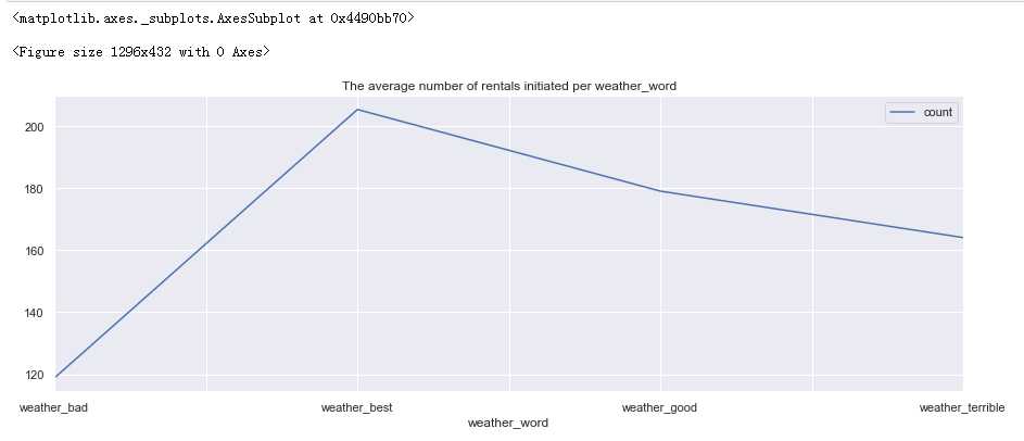
分析:
租车人数受天气好坏影响很大
6.4.4 风速
风速对出行情况的影响
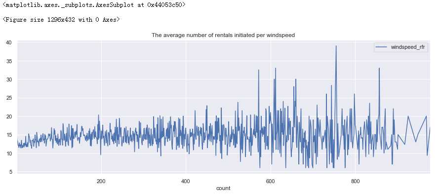
先来看下两年时间风速的变化趋势
#设置画框尺寸
fig = plt.figure(figsize=(18,6))
day_df = full_X_1.groupby([‘count‘], as_index=True).agg({‘windspeed_rfr‘:‘mean‘})
day_df.plot(figsize=(15,5),title = ‘The average number of rentals initiated per windspeed‘)
观察一下租赁人数随风速变化趋势,考虑到风速特别大的时候很少,如果取平均值会出现异常,所以按风速对租赁数量取最大值。
fig = plt.figure(figsize=(18,6))
windspeed_rentals = full_X_1.groupby([‘windspeed‘], as_index=True).agg({‘count‘:‘max‘})
windspeed_rentals .plot(figsize=(15,5),title = ‘Max number of rentals initiated per hour in different windspeed‘)
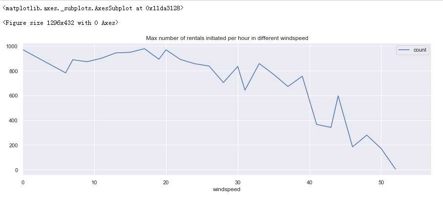
分析:
大于20租车数量降低,小于20租车人数始终保持在较高数量
6.4.5湿度humidity
fig = plt.figure(figsize=(18,6))
windspeed_rentals = full_X_1.groupby([‘humidity‘], as_index=True).agg({‘count‘:‘mean‘})
windspeed_rentals .plot(figsize=(15,5),title = ‘Max number of rentals initiated per hour in different humidity‘)
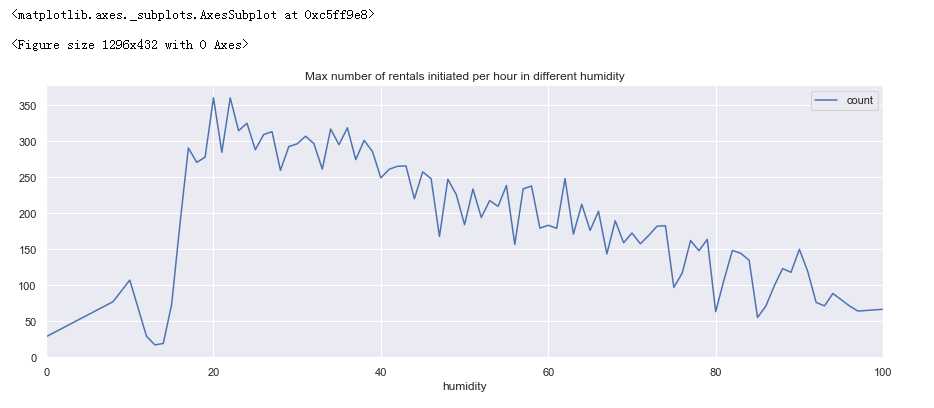
分析:
湿度为20租车人数出现峰值,大于20之后随之降低
6.4.6温度temp
fig = plt.figure(figsize=(18,6))
windspeed_rentals = full_X_1.groupby([‘temp‘], as_index=True).agg({‘count‘:‘mean‘})
windspeed_rentals .plot(figsize=(15,5),title = ‘Max number of rentals initiated per hour in different temp ‘)
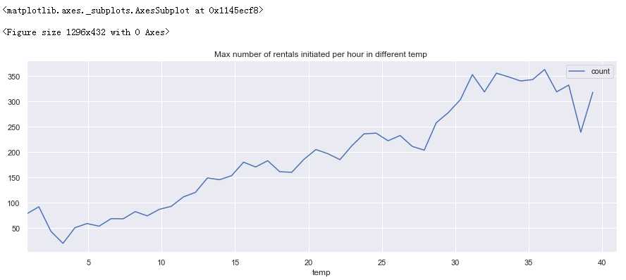
分析:
0-35度租车数量随着温度的升高而增加
35度后租车人数随温度的升高而减少
6.4.6体表温度atemp
fig = plt.figure(figsize=(18,6))
windspeed_rentals = full_X_1.groupby([‘atemp‘], as_index=True).agg({‘count‘:‘mean‘})
windspeed_rentals .plot(figsize=(15,5),title = ‘Max number of rentals initiated per hour in different atemp ‘)
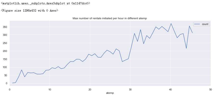
分析:
0-40度租车数量随着体表温度的升高而增加
40度后租车人数随体表温度的升高而减少
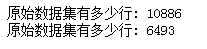
#原始数据集有891行
sourceRow=10886
#原始数据集:特征
source_X = full_X.loc[0:sourceRow-1,:]

#原始数据集:标签
source_y = full.loc[0:sourceRow-1,‘count‘]

#预测数据集:特征
pred_X = full_X.loc[sourceRow:,:]
‘‘‘
确保这里原始数据集取的是前891行的数据,不然后面模型会有错误
‘‘‘
#原始数据集有多少行
print(‘原始数据集有多少行:‘,source_X.shape[0])
#预测数据集大小
print(‘原始数据集有多少行:‘,pred_X.shape[0])
7.1 建立训练数据集和测试数据集
from sklearn.model_selection import train_test_split

#建立模型用的训练数据集和测试数据集
train_X, test_X, train_y, test_y = train_test_split(source_X ,
                                                    source_y,
                                                    train_size=0.8)

#输出数据集大小
print (‘原始数据集特征:‘,source_X.shape,
       ‘训练数据集特征:‘,train_X.shape,
      ‘测试数据集特征:‘,test_X.shape)

print (‘原始数据集标签:‘,source_y.shape,
       ‘训练数据集标签:‘,train_y.shape,
      ‘测试数据集标签:‘,test_y.shape)

7.2 训练模型
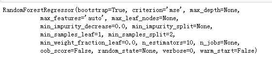
随机森林回归
#第1步:导入算法
from sklearn.ensemble import RandomForestRegressor
#第2步:创建模型:逻辑回归(logisic regression)
model = RandomForestRegressor()
#第3步:训练模型
model.fit( train_X , train_y )
7.3评估模型
model.score(test_X , test_y )
pred_Y = model.predict(pred_X)

‘‘‘
生成的预测值是浮点数(0.0,1,0)
但是Kaggle要求提交的结果是整型(0,1)
所以要对数据类型进行转换
‘‘‘
pred_Y=pred_Y.astype(int)
#乘客id

# data = full_X.loc[sourceRow:,[‘hour‘,‘temp‘,‘atemp‘,‘year‘,‘month‘,‘seaon_spring‘,‘season_summer‘,‘season_autumn‘,‘season_winter‘
#                                     ,‘weather_best‘,‘weather_good‘,‘weather_bad‘,‘weather_terrible‘,‘humidity‘,‘windspeed‘]]

# frame2 = pd.DataFrame(data,index=[‘one‘,‘two‘,‘three‘,‘four‘,‘five‘],columns=[‘year‘,‘state‘,‘pop‘,‘debt‘])
datatime = bikeDf.loc[sourceRow:,[‘datetime‘]]

li = []
for i in range(10886,17379):
    li.append(i)


#数据框:乘客id,预测生存情况的值
pred = pd.DataFrame(
     {‘count‘: pred_Y},index=li)
#10886

predDf = pd.concat([datatime,pred],axis=1)

predDf.shape
predDf.head()
#保存结果
predDf.to_csv( ‘bike_pred.csv‘ , index = False )
对于相关性高的特征值
1、时间hour :每天上下班时间是两个用车高峰,而中午也会有一个小高峰,一个是上午8点、一个是下午17点
2、时间year :租车数量逐年提升
3、月份month 、季节season 租车数量集中在5-10月,租车重数在夏天和秋天
4、天气wheather :天气好坏直接影响租车数量
5、风速windspeed :大于20租车数量降低,小于20租车人数始终保持在较高数量
6、湿度humidity :湿度为20租车人数出现峰值,大于20之后随之降低
7、温度temp :
0-35度租车数量随着温度的升高而增加
35度后租车人数随温度的升高而减少
8、体表温度atemp:
0-40度租车数量随着体表温度的升高而增加
40度后租车人数随体表温度的升高而减少
建议:
一、对于租车公司:
重点运营集中在:
1、上下班高峰期
2、重点季节是夏季和秋季、重点月份5-10月
对于淡季:
1、要重点营销,采取优惠,月卡等优惠手段促进租车数量
2、做好共享单车的保养等后勤工作
二、对于个人
明确单车使用高峰期,提前做好准备,以免耽误正常出行
(●‘?‘●)如果对您有用,别忘了点个赞鼓励一下~
标签:数据分析 datetime 数据可视化 过程 diff get 夏天 title day
原文地址:https://www.cnblogs.com/foremostxl/p/12058954.html