标签:actor fonts 不执行 enumerate point 缺失值 statistic reset 坐标
项目目的:利用车贷金融数据建立评分卡,并尝试多次迭代观察不同行为对模型,以及建模中间过程产生哪些影响。
首先是标准化导入需要使用的工具
import pandas as pd
import numpy as np
import matplotlib.pyplot as plt
plt.style.use("ggplot")#风格设置
import seaborn as sns
sns.set_style("whitegrid")
%matplotlib inline
import warnings #忽略错误模块
warnings.filterwarnings("ignore")
plt.rcParams["font.sans-serif"]=["SimHei"] #指定默认字体
导入需要的数据
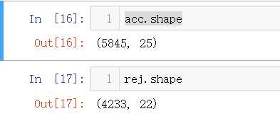
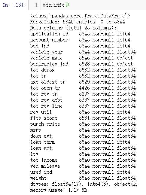
acc = pd.read_csv(‘accepts.csv‘)  #通过的客户
rej = pd.read_csv(‘rejects.csv‘)  #拒绝的客户
pd.set_option("display.max_columns",len(acc.columns))#解决全部显示的问题
acc.head()
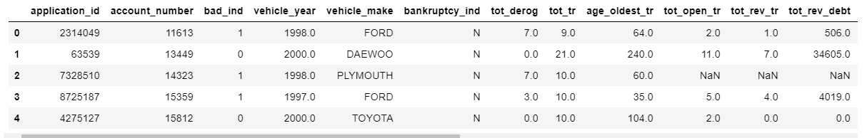
各变量含义介绍: #中文含义
#中文含义
##application_id---申请者ID
##account_number---帐户号
##bad_ind---是否违约
##vehicle_year---汽车购买时间
##vehicle_make---汽车制造商
##bankruptcy_ind---曾经破产标识
##tot_derog---五年内信用不良事件数量(比如手机欠费消号)
##tot_tr---全部帐户数量
##age_oldest_tr---最久账号存续时间(月)
##tot_open_tr---在使用帐户数量
##tot_rev_tr---在使用可循环贷款帐户数量(比如信用卡)
##tot_rev_debt---在使用可循环贷款帐户余额(比如信用卡欠款)
##tot_rev_line---可循环贷款帐户限额(信用卡授权额度)
##rev_util---可循环贷款帐户使用比例(余额/限额)
##fico_score---FICO打分
##purch_price---汽车购买金额(元)
##msrp---建议售价
##down_pyt---分期付款的首次交款
##loan_term---贷款期限(月)
##loan_amt---贷款金额
##ltv---贷款金额/建议售价*100
##tot_income---月均收入(元)
##veh_mileage---行使历程(Mile)
##used_ind---是否使用
##weight---样本权重
数据清洗
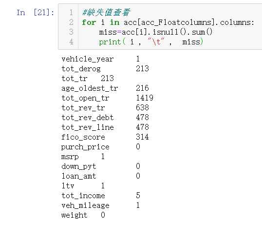
1.缺失值处理
数值数据处理
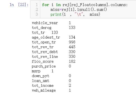
acc_Floatcolumns=[i for i in acc.columns if acc[i].dtype=="float"]
rej_Floatcolumns=[i for i in rej.columns if rej[i].dtype=="float"]
利用Imputer 模块进行缺失值填充

from sklearn.preprocessing import Imputer#只支持 均值,中位数,众数填补
inputer = Imputer(missing_values = ‘NaN‘, strategy = ‘mean‘, axis = 0)
inputer = inputer.fit(X)
X = inputer.transform(X)
主要参数说明:
missing_values:缺失值,可以为整数或NaN(缺失值numpy.nan用字符串‘NaN’表示),默认为NaN

strategy:替换策略,字符串,默认用均值‘mean’替换

①若为mean时,用特征列的均值替换

②若为median时,用特征列的中位数替换

③若为most_frequent时,用特征列的众数替换

axis:指定轴数,默认axis=0代表列,axis=1代表行

copy:设置为True代表不在原数据集上修改,设置为False时,就地修改,存在如下情况时,即使设置为False时,也不会就地修改

①X不是浮点值数组

②X是稀疏且missing_values=0

③axis=0且X为CRS矩阵

④axis=1且X为CSC矩阵

statistics_属性:axis设置为0时,每个特征的填充值数组,axis=1时,报没有该属性错误
from sklearn.preprocessing import Imputer
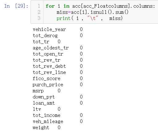
#数值信息缺失值处理
inputer=Imputer(missing_values=‘NaN‘, strategy=‘mean‘, axis=0) #均值填充,列
inputer=inputer.fit(acc[acc_Floatcolumns])# 计算
acc[acc_Floatcolumns] = inputer.transform(acc[acc_Floatcolumns]) #引用
inputer=Imputer(missing_values=‘NaN‘, strategy=‘mean‘, axis=0) #均值填充,列
inputer=inputer.fit(rej[rej_Floatcolumns])# 计算
rej[rej_Floatcolumns] = inputer.transform(rej[rej_Floatcolumns]) #引用
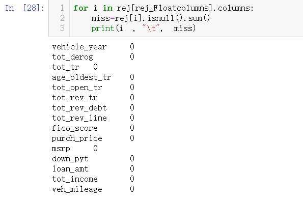
for i in rej_Floatcolumns:
    rej[i]=acc[i].fillna(rej[i].mean())
#mean()均值
#mode()众数
#median()中位数
数值型数据缺失值填充完毕
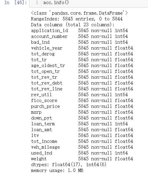
#分类信息缺失值数据处理
acc_objectcolumns=[i for i in acc.columns if acc[i].dtype=="object"]
rej_objectcolumns=[i for i in rej.columns if rej[i].dtype=="object"]
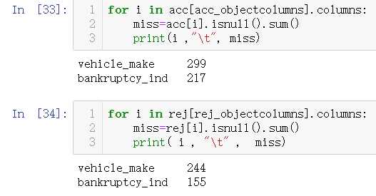
两个数据为汽车制造商与曾经破产标志,这里删除汽车制造商。
#删除汽车制造商特征
acc.drop(columns="vehicle_make",axis=0,inplace=True)
rej.drop(columns="vehicle_make",axis=0,inplace=True)
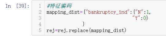
对于破产可以单独一类归纳,但在这里占比实在太小,没太大意义,所以直接替换成N代替
#空值替换成N
acc["bankruptcy_ind"]=acc["bankruptcy_ind"].fillna("N")
rej["bankruptcy_ind"]=rej["bankruptcy_ind"].fillna("N")
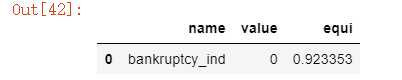
同值信息处理:
一般如果某一项特征超过90%都是同一种信息,那么一般对模型将毫无作用,所以优先删除这一变量。
#同值信息处理
from scipy.stats import mode
equ_fea=[]
for i in acc.columns:
        mode_value=mode(acc[i])[0][0] #求众数值
        mode_rate=mode(acc[i])[1][0]/acc.shape[0]#求得众数占比
        if mode_rate >0.9:
            equ_fea.append([i,mode_value,mode_rate])
dt=pd.DataFrame(equ_fea,columns=["name","value","equi"])
dt.sort_values(by="equi")
删除处理
acc.drop(columns="bankruptcy_ind",axis=0,inplace=True)
rej.drop(columns="bankruptcy_ind",axis=0,inplace=True)
#借款期限描述
cla=["loan_term"]
for i in cla:
    pvt=pd.pivot_table(acc[["bad_ind",i]],index=i,columns="bad_ind",aggfunc=len)
    pvt.plot(kind="bar")
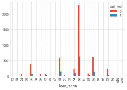
借款期限分布符合一般规律,逾期比列方面没有太大区别
cel=[i for i in acc.columns if acc[i].dtypes =="float"]
for i ,j in enumerate(cel):
    plt.figure(figsize=(8,5*len(cel)))
    plt.subplot(len(cel),1,i+1)
    sns.distplot(acc[j][acc.bad_ind==0],color="b")
    sns.distplot(acc[j][acc.bad_ind==1],color="r")
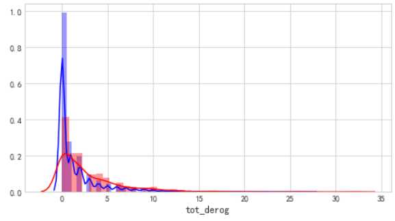
具备不良信息的客户,占比接近40%,次数越多,相对的逾期客户越多
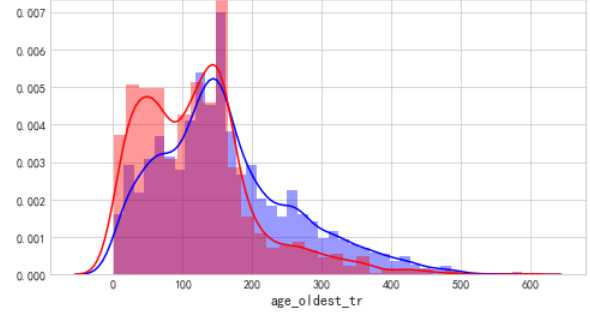
从账龄来看,账龄越短,逾期人数越多,逾期概率也越高
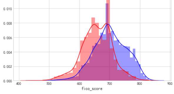
FICO评分,呈现正太分布,并且能够看见,评分越低逾期率越高,700分为分界,得分越高逾期率越低,评分效果是比较显著的
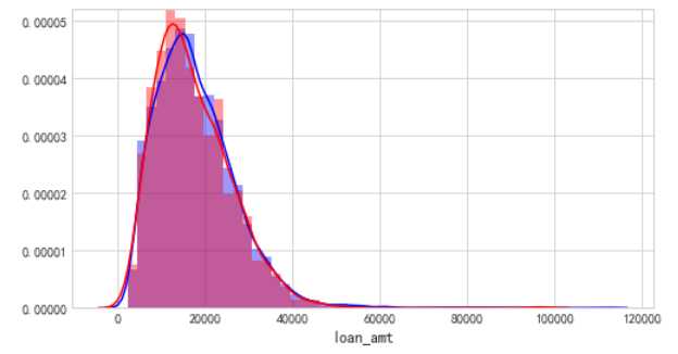
借款金额多集中在4万一下,呈现正太分布
拒绝推断
#一般情况下如果我们只拿申请通过的样本建立评分卡,会出现样本偏差,不能很好适用于整个申请人群,同时也方便评分卡覆盖之前的决策影响。
#这里采用K-NN做拒绝推断
1.取出部分变量用于做KNN:由于KNN算法要求使用连续变量,因此仅选了部分重要的连续变量用于做KNN模型
acc_x = acc[["tot_derog","age_oldest_tr","rev_util","fico_score","ltv"]]
acc_y = acc[‘bad_ind‘]
rej_x = rej[["tot_derog","age_oldest_tr","rev_util","fico_score","ltv"]]
#数据标准化
def MaxMinNormalization(dataset):
    maxdf=dataset.max()
    mindf=dataset.min()
    normal=(dataset-mindf) / (maxdf-mindf)
    return normal
acc_x_norm =MaxMinNormalization(acc_x)
rej_x_norm =MaxMinNormalization(rej_x)
 #利用knn模型进行预测,做拒绝推断
from sklearn.neighbors import NearestNeighbors
from sklearn.neighbors import KNeighborsClassifier
neigh = KNeighborsClassifier(n_neighbors=5, weights=‘distance‘)
neigh.fit(acc_x_norm, acc_y)

rej[‘bad_ind‘] = neigh.predict(rej_x_norm)
#删除ID
rej.drop(columns="application_id",axis=0,inplace=True)
#将审核通过的申请者和未通过的申请者进行合并
# accepts的数据是针对于违约用户的过度抽样
#因此,rejects也要进行同样比例的抽样
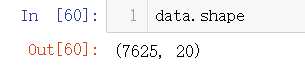
rej_res = rej[rej[‘bad_ind‘] == 0].sample(1340)
rej_res = pd.concat([rej_res, rej[rej[‘bad_ind‘] == 1]], axis = 0)
data = pd.concat([acc, rej_res], axis=0)
建模数据准备
#盖帽法处理年份变量中的异常值,并将年份其转化为距现在多长时间
year_min = data.vehicle_year.quantile(0.1) #求得分位数
year_max = data.vehicle_year.quantile(0.99)
data.vehicle_year = data.vehicle_year.map(lambda x: year_min if x <= year_min else x)
data.vehicle_year = data.vehicle_year.map(lambda x: year_max if x >= year_max else x)
data.vehicle_year = data.vehicle_year.map(lambda x: 2019 - x)
#盖帽法处理所有数值型数据的异常值
dist=["age_oldest_tr","down_pyt","fico_score","loan_amt","loan_term","ltv","msrp","purch_price",
     "rev_util","tot_income","tot_rev_debt","tot_rev_line","tot_tr","veh_mileage"]
for i in dist:
    i_min=data[i].quantile(0.1)
    i_max=data[i].quantile(0.99)
    data[i]=data[i].map(lambda x : i_min if x <= i_min else x)
    data[i]=data[i].map(lambda x : i_max if x >= i_max else x)
#划分 x与y
x_list=list(data.columns)
x_list.remove("bad_ind") #再x_list中剔除 bad_ind 变量
x=data[x_list]
y=data["bad_ind"]
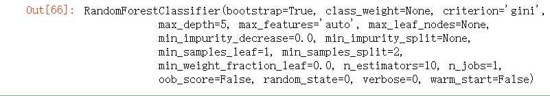
#利用随机森林选择GINI系数排名靠前的变量
from sklearn.ensemble import RandomForestClassifier
clf = RandomForestClassifier(max_depth=5, random_state=0)
clf.fit(x,y)
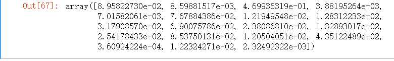
#返回变量的GINI系数
clf.feature_importances_
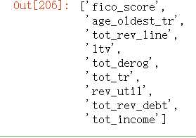
#选择排名前9的特征
importances = list(clf.feature_importances_)
importances_order = importances.copy()
importances_order.sort(reverse=True)

cols = list(x.columns)
col_top = []
for i in importances_order[:9]:
    col_top.append((i,cols[importances.index(i)]))
col_top
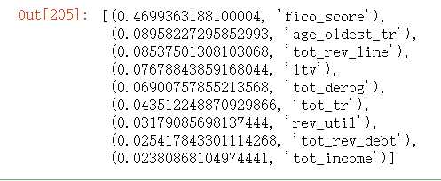
#截取columns
col=[i[1] for i in col_top]
col
#开始进行特征分箱
import numpy as np
import pandas as pd
from sklearn.metrics import confusion_matrix
1.卡方分箱
def SplitData(df, col, numOfSplit, special_attribute=[]):
    ‘‘‘
    :param df: 按照col排序后的数据集
    :param col: 待分箱的变量
    :param numOfSplit: 切分的组别数
    :param special_attribute: 在切分数据集的时候,某些特殊值需要排除在外
    :return: 在原数据集上增加一列,把原始细粒度的col重新划分成粗粒度的值,便于分箱中的合并处理
    ‘‘‘
    df2 = df.copy()
    if special_attribute != []:
        df2 = df.loc[~df[col].isin(special_attribute)]
    N = df2.shape[0]
    n = int(N/numOfSplit)
    splitPointIndex = [i*n for i in range(1,numOfSplit)]
    rawValues = sorted(list(df2[col]))
    splitPoint = [rawValues[i] for i in splitPointIndex]
    splitPoint = sorted(list(set(splitPoint)))
    return splitPoint

def MaximumBinPcnt(df,col):
    ‘‘‘
    :return: 数据集df中,变量col的分布占比
    ‘‘‘
    N = df.shape[0]
    total = df.groupby([col])[col].count()
    pcnt = total*1.0/N
    return max(pcnt)
def Chi2(df, total_col, bad_col):
    ‘‘‘
    :param df: 包含全部样本总计与坏样本总计的数据框
    :param total_col: 全部样本的个数
    :param bad_col: 坏样本的个数
    :return: 卡方值
    ‘‘‘
    df2 = df.copy()
    # 求出df中,总体的坏样本率和好样本率
    badRate = sum(df2[bad_col])*1.0/sum(df2[total_col])
    # 当全部样本只有好或者坏样本时,卡方值为0
    if badRate in [0,1]:
        return 0
    df2[‘good‘] = df2.apply(lambda x: x[total_col] - x[bad_col], axis = 1)
    goodRate = sum(df2[‘good‘]) * 1.0 / sum(df2[total_col])
    # 期望坏(好)样本个数=全部样本个数*平均坏(好)样本占比
    df2[‘badExpected‘] = df[total_col].apply(lambda x: x*badRate)
    df2[‘goodExpected‘] = df[total_col].apply(lambda x: x * goodRate)
    badCombined = zip(df2[‘badExpected‘], df2[bad_col])
    goodCombined = zip(df2[‘goodExpected‘], df2[‘good‘])
    badChi = [(i[0]-i[1])**2/i[0] for i in badCombined]
    goodChi = [(i[0] - i[1]) ** 2 / i[0] for i in goodCombined]
    chi2 = sum(badChi) + sum(goodChi)
    return chi2

def BinBadRate(df, col, target, grantRateIndicator=0):
    ‘‘‘
    :param df: 需要计算好坏比率的数据集
    :param col: 需要计算好坏比率的特征
    :param target: 好坏标签
    :param grantRateIndicator: 1返回总体的坏样本率,0不返回
    :return: 每箱的坏样本率,以及总体的坏样本率(当grantRateIndicator==1时)
    ‘‘‘
    total = df.groupby([col])[target].count()
    total = pd.DataFrame({‘total‘: total})
    bad = df.groupby([col])[target].sum()
    bad = pd.DataFrame({‘bad‘: bad})
    regroup = total.merge(bad, left_index=True, right_index=True, how=‘left‘)
    regroup.reset_index(level=0, inplace=True)
    regroup[‘bad_rate‘] = regroup.apply(lambda x: x.bad / x.total, axis=1)
    dicts = dict(zip(regroup[col],regroup[‘bad_rate‘]))
    if grantRateIndicator==0:
        return (dicts, regroup)
    N = sum(regroup[‘total‘])
    B = sum(regroup[‘bad‘])
    overallRate = B * 1.0 / N
    return (dicts, regroup, overallRate)

def AssignGroup(x, bin):
    ‘‘‘
    :return: 数值x在区间映射下的结果。例如,x=2,bin=[0,3,5], 由于0<x<3,x映射成3
    ‘‘‘
    N = len(bin)
    if x<=min(bin):
        return min(bin)
    elif x>max(bin):
        return 10e10
    else:
        for i in range(N-1):
            if bin[i] < x <= bin[i+1]:
                return bin[i+1]

def AssignBin(x, cutOffPoints,special_attribute=[]):
    ‘‘‘
    :param x: 某个变量的某个取值
    :param cutOffPoints: 上述变量的分箱结果,用切分点表示
    :param special_attribute:  不参与分箱的特殊取值
    :return: 分箱后的对应的第几个箱,从0开始
    例如, cutOffPoints = [10,20,30], 对于 x = 7, 返回 Bin 0;对于x=23,返回Bin 2; 对于x = 35, return Bin 3。
    对于特殊值,返回的序列数前加"-"
    ‘‘‘
    cutOffPoints2 = [i for i in cutOffPoints if i not in special_attribute]
    numBin = len(cutOffPoints2)
    if x in special_attribute:
        i = special_attribute.index(x)+1
        return ‘Bin {}‘.format(0-i)
    if x<=cutOffPoints2[0]:
        return ‘Bin 0‘
    elif x > cutOffPoints2[-1]:
        return ‘Bin {}‘.format(numBin)
    else:
        for i in range(0,numBin):
            if cutOffPoints2[i] < x <=  cutOffPoints2[i+1]:
                return ‘Bin {}‘.format(i+1)
def ChiMerge(df, col, target, max_interval=5,special_attribute=[],minBinPcnt=0):
    ‘‘‘
    :param df: 包含目标变量与分箱属性的数据框
    :param col: 需要分箱的属性
    :param target: 目标变量,取值0或1
    :param max_interval: 最大分箱数。如果原始属性的取值个数低于该参数,不执行这段函数
    :param special_attribute: 不参与分箱的属性取值
    :param minBinPcnt:最小箱的占比,默认为0
    :return: 分箱结果
    ‘‘‘
    colLevels = sorted(list(set(df[col])))
    N_distinct = len(colLevels)
    if N_distinct <= max_interval:  #如果原始属性的取值个数低于max_interval,不执行这段函数
        print("The number of original levels for {} is less than or equal to max intervals".format(col))
        return colLevels[:-1]
    else:
        if len(special_attribute)>=1:
            df1 = df.loc[df[col].isin(special_attribute)]
            df2 = df.loc[~df[col].isin(special_attribute)]
        else:
            df2 = df.copy()
        N_distinct = len(list(set(df2[col])))

        # 步骤一: 通过col对数据集进行分组,求出每组的总样本数与坏样本数
        if N_distinct > 100:
            split_x = SplitData(df2, col, 100)
            df2[‘temp‘] = df2[col].map(lambda x: AssignGroup(x, split_x))
        else:
            df2[‘temp‘] = df2[col]
        # 总体bad rate将被用来计算expected bad count
        (binBadRate, regroup, overallRate) = BinBadRate(df2, ‘temp‘, target, grantRateIndicator=1)

        # 首先,每个单独的属性值将被分为单独的一组
        # 对属性值进行排序,然后两两组别进行合并
        colLevels = sorted(list(set(df2[‘temp‘])))
        groupIntervals = [[i] for i in colLevels]

        # 步骤二:建立循环,不断合并最优的相邻两个组别,直到:
        # 1,最终分裂出来的分箱数<=预设的最大分箱数
        # 2,每箱的占比不低于预设值(可选)
        # 3,每箱同时包含好坏样本
        # 如果有特殊属性,那么最终分裂出来的分箱数=预设的最大分箱数-特殊属性的个数
        split_intervals = max_interval - len(special_attribute)
        while (len(groupIntervals) > split_intervals):  # 终止条件: 当前分箱数=预设的分箱数
            # 每次循环时, 计算合并相邻组别后的卡方值。具有最小卡方值的合并方案,是最优方案
            chisqList = []
            for k in range(len(groupIntervals)-1):
                temp_group = groupIntervals[k] + groupIntervals[k+1]
                df2b = regroup.loc[regroup[‘temp‘].isin(temp_group)]
                chisq = Chi2(df2b, ‘total‘, ‘bad‘)
                chisqList.append(chisq)
            best_comnbined = chisqList.index(min(chisqList))
            groupIntervals[best_comnbined] = groupIntervals[best_comnbined] + groupIntervals[best_comnbined+1]
            # 当将最优的相邻的两个变量合并在一起后,需要从原来的列表中将其移除。例如,将[3,4,5] 与[6,7]合并成[3,4,5,6,7]后,需要将[3,4,5] 与[6,7]移除,保留[3,4,5,6,7]
            groupIntervals.remove(groupIntervals[best_comnbined+1])
        groupIntervals = [sorted(i) for i in groupIntervals]
        cutOffPoints = [max(i) for i in groupIntervals[:-1]]

        # 检查是否有箱没有好或者坏样本。如果有,需要跟相邻的箱进行合并,直到每箱同时包含好坏样本
        groupedvalues = df2[‘temp‘].apply(lambda x: AssignBin(x, cutOffPoints))
        df2[‘temp_Bin‘] = groupedvalues
        (binBadRate,regroup) = BinBadRate(df2, ‘temp_Bin‘, target)
        [minBadRate, maxBadRate] = [min(binBadRate.values()),max(binBadRate.values())]
        while minBadRate ==0 or maxBadRate == 1:
            # 找出全部为好/坏样本的箱
            indexForBad01 = regroup[regroup[‘bad_rate‘].isin([0,1])].temp_Bin.tolist()
            bin=indexForBad01[0]
            # 如果是最后一箱,则需要和上一个箱进行合并,也就意味着分裂点cutOffPoints中的最后一个需要移除
            if bin == max(regroup.temp_Bin):
                cutOffPoints = cutOffPoints[:-1]
            # 如果是第一箱,则需要和下一个箱进行合并,也就意味着分裂点cutOffPoints中的第一个需要移除
            elif bin == min(regroup.temp_Bin):
                cutOffPoints = cutOffPoints[1:]
            # 如果是中间的某一箱,则需要和前后中的一个箱进行合并,依据是较小的卡方值
            else:
                # 和前一箱进行合并,并且计算卡方值
                currentIndex = list(regroup.temp_Bin).index(bin)
                prevIndex = list(regroup.temp_Bin)[currentIndex - 1]
                df3 = df2.loc[df2[‘temp_Bin‘].isin([prevIndex, bin])]
                (binBadRate, df2b) = BinBadRate(df3, ‘temp_Bin‘, target)
                chisq1 = Chi2(df2b, ‘total‘, ‘bad‘)
                # 和后一箱进行合并,并且计算卡方值
                laterIndex = list(regroup.temp_Bin)[currentIndex + 1]
                df3b = df2.loc[df2[‘temp_Bin‘].isin([laterIndex, bin])]
                (binBadRate, df2b) = BinBadRate(df3b, ‘temp_Bin‘, target)
                chisq2 = Chi2(df2b, ‘total‘, ‘bad‘)
                if chisq1 < chisq2:
                    cutOffPoints.remove(cutOffPoints[currentIndex - 1])
                else:
                    cutOffPoints.remove(cutOffPoints[currentIndex])
            # 完成合并之后,需要再次计算新的分箱准则下,每箱是否同时包含好坏样本
            groupedvalues = df2[‘temp‘].apply(lambda x: AssignBin(x, cutOffPoints))
            df2[‘temp_Bin‘] = groupedvalues
            (binBadRate, regroup) = BinBadRate(df2, ‘temp_Bin‘, target)
            [minBadRate, maxBadRate] = [min(binBadRate.values()), max(binBadRate.values())]
        # 需要检查分箱后的最小占比
        if minBinPcnt > 0:
            groupedvalues = df2[‘temp‘].apply(lambda x: AssignBin(x, cutOffPoints))
            df2[‘temp_Bin‘] = groupedvalues
            valueCounts = groupedvalues.value_counts().to_frame()
            N = sum(valueCounts[‘temp‘])
            valueCounts[‘pcnt‘] = valueCounts[‘temp‘].apply(lambda x: x * 1.0 / N)
            valueCounts = valueCounts.sort_index()
            minPcnt = min(valueCounts[‘pcnt‘])
            while minPcnt < minBinPcnt and len(cutOffPoints) > 2:
                # 找出占比最小的箱
                indexForMinPcnt = valueCounts[valueCounts[‘pcnt‘] == minPcnt].index.tolist()[0]
                # 如果占比最小的箱是最后一箱,则需要和上一个箱进行合并,也就意味着分裂点cutOffPoints中的最后一个需要移除
                if indexForMinPcnt == max(valueCounts.index):
                    cutOffPoints = cutOffPoints[:-1]
                # 如果占比最小的箱是第一箱,则需要和下一个箱进行合并,也就意味着分裂点cutOffPoints中的第一个需要移除
                elif indexForMinPcnt == min(valueCounts.index):
                    cutOffPoints = cutOffPoints[1:]
                # 如果占比最小的箱是中间的某一箱,则需要和前后中的一个箱进行合并,依据是较小的卡方值
                else:
                    # 和前一箱进行合并,并且计算卡方值
                    currentIndex = list(valueCounts.index).index(indexForMinPcnt)
                    prevIndex = list(valueCounts.index)[currentIndex - 1]
                    df3 = df2.loc[df2[‘temp_Bin‘].isin([prevIndex, indexForMinPcnt])]
                    (binBadRate, df2b) = BinBadRate(df3, ‘temp_Bin‘, target)
                    chisq1 = Chi2(df2b, ‘total‘, ‘bad‘)
                    # 和后一箱进行合并,并且计算卡方值
                    laterIndex = list(valueCounts.index)[currentIndex + 1]
                    df3b = df2.loc[df2[‘temp_Bin‘].isin([laterIndex, indexForMinPcnt])]
                    (binBadRate, df2b) = BinBadRate(df3b, ‘temp_Bin‘, target)
                    chisq2 = Chi2(df2b, ‘total‘, ‘bad‘)
                    if chisq1 < chisq2:
                        cutOffPoints.remove(cutOffPoints[currentIndex - 1])
                    else:
                        cutOffPoints.remove(cutOffPoints[currentIndex])
                groupedvalues = df2[‘temp‘].apply(lambda x: AssignBin(x, cutOffPoints))
                df2[‘temp_Bin‘] = groupedvalues
                valueCounts = groupedvalues.value_counts().to_frame()
                valueCounts[‘pcnt‘] = valueCounts[‘temp‘].apply(lambda x: x * 1.0 / N)
                valueCounts = valueCounts.sort_index()
                minPcnt = min(valueCounts[‘pcnt‘])
        cutOffPoints = special_attribute + cutOffPoints
        return cutOffPoints
def ChiMerge(df, col, target, max_interval=5,special_attribute=[],minBinPcnt=0):
    ‘‘‘
    :param df: 包含目标变量与分箱属性的数据框
    :param col: 需要分箱的属性
    :param target: 目标变量,取值0或1
    :param max_interval: 最大分箱数。如果原始属性的取值个数低于该参数,不执行这段函数
    :param special_attribute: 不参与分箱的属性取值
    :param minBinPcnt:最小箱的占比,默认为0
    :return: 分箱结果
分别采用最小箱占比 0 和 0.5 进行两次分箱方便后续对比结果
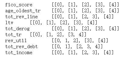
#最小箱占比0
df_dist={}
for i in col:
    df_feat=ChiMerge(data,i, "bad_ind", max_interval=5,special_attribute=[],minBinPcnt=0)
    df_dist[i]=df_feat
print (df_dist)

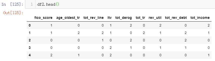
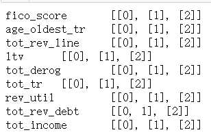
#最小箱占比0.5
df_dist={}
for i in col:
    df_feat=ChiMerge(data,i, "bad_ind", max_interval=5,special_attribute=[],minBinPcnt=0.5)
    df_dist[i]=df_feat
print (df_dist)

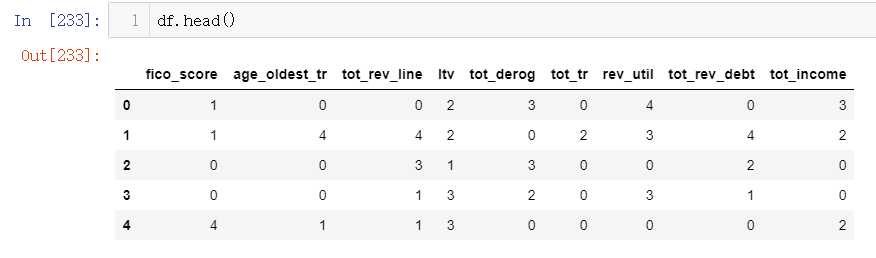
#采用pd.cut()划分数据
def box_col_to_df(to_box,col,num_b):#数据集    需要转换的数据列   切割点LISI
    bins=[-100.0]+num_b+[1000000000.0] #因为pd.cut()是封闭的,这里把bins的上下区间扩大
    to_box[col]=pd.cut(to_box[col],bins=bins,include_lowest=True,labels=range(len(bins)-1))
df=data[col]
for i in col:
    box_col_to_df(df,i,df_dist[i])
df2=data[col]
for i in col:
    box_col_to_df(df2,i,df_dist[i])
#计算woe 和IV 值
def CalcWOE(df, col, target):
    ‘‘‘
    :param df: 包含需要计算WOE的变量和目标变量
    :param col: 需要计算WOE、IV的变量,必须是分箱后的变量,或者不需要分箱的类别型变量
    :param target: 目标变量,0、1表示好、坏
    :return: 返回WOE和IV
    ‘‘‘
    total = df.groupby([col])[target].count()
    total = pd.DataFrame({‘total‘: total})
    bad = df.groupby([col])[target].sum()
    bad = pd.DataFrame({‘bad‘: bad})
    regroup = total.merge(bad, left_index=True, right_index=True, how=‘left‘)
    regroup.reset_index(level=0, inplace=True)
    N = sum(regroup[‘total‘])
    B = sum(regroup[‘bad‘])
    regroup[‘good‘] = regroup[‘total‘] - regroup[‘bad‘]
    G = N - B
    regroup[‘bad_pcnt‘] = regroup[‘bad‘].map(lambda x: x*1.0/B)
    regroup[‘good_pcnt‘] = regroup[‘good‘].map(lambda x: x * 1.0 / G)
    regroup[‘WOE‘] = regroup.apply(lambda x: np.log(x.good_pcnt*1.0/x.bad_pcnt),axis = 1)
    WOE_dict = regroup[[col,‘WOE‘]].set_index(col).to_dict(orient=‘index‘)
    for k, v in WOE_dict.items():
        WOE_dict[k] = v[‘WOE‘]
    IV = regroup.apply(lambda x: (x.good_pcnt-x.bad_pcnt)*np.log(x.good_pcnt*1.0/x.bad_pcnt),axis = 1)
    IV = sum(IV)
    return {"WOE": WOE_dict, ‘IV‘:IV}
df["bad_ind"]=data["bad_ind"]
df2["bad_ind"]=data["bad_ind"]
iv=[]
IV={}
WOE={}
for i in col:
    df_dist=CalcWOE(df, i, "bad_ind")
    IV[i]=df_dist["IV"]
    iv.append([i,df_dist["IV"]])
    WOE[i]=df_dist["WOE"]
lis=pd.DataFrame(iv,columns=["name","iv"])
print(IV)
print(WOE)
print(lis
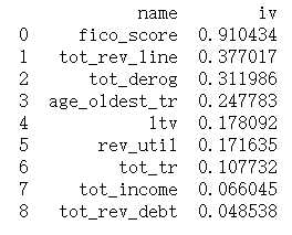
iv=[]
IV={}
WOE={}
for i in col:
    df_dist=CalcWOE(df2, i, "bad_ind")
    IV[i]=df_dist["IV"]
    iv.append([i,df_dist["IV"]])
    WOE[i]=df_dist["WOE"]
lis=pd.DataFrame(iv,columns=["name","iv"])
print(IV)
print(WOE)
print(lis)
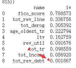
可见分箱方案的选择对IV值存在较直接的影响,实际操作中需要结合实际经验不断迭代。
 ‘‘‘
    :return: 返回序列x中有几个元素不满足单调性,以及这些元素的位置。
    例如,x=[1,3,2,5], 元素3比前后两个元素都大,不满足单调性;元素2比前后两个元素都小,也不满足单调性。
    故返回的不满足单调性的元素个数为2,位置为1和2.
    ‘‘‘
    monotone = [x[i]<x[i+1] and x[i] < x[i-1] or x[i]>x[i+1] and x[i] > x[i-1] for i in range(1,len(x)-1)]
    index_of_nonmonotone = [i+1 for i in range(len(monotone)) if monotone[i]]
    return {‘count_of_nonmonotone‘:monotone.count(True), ‘index_of_nonmonotone‘:index_of_nonmonotone}

## 判断某变量的坏样本率是否单调
def BadRateMonotone(df, sortByVar, target,special_attribute = []):
    ‘‘‘
    :param df: 包含检验坏样本率的变量,和目标变量
    :param sortByVar: 需要检验坏样本率的变量
    :param target: 目标变量,0、1表示好、坏
    :param special_attribute: 不参与检验的特殊值
    :return: 坏样本率单调与否
    ‘‘‘
    df2 = df.loc[~df[sortByVar].isin(special_attribute)]
    if len(set(df2[sortByVar])) <= 2:
        return True
    regroup = BinBadRate(df2, sortByVar, target)[1]
    combined = zip(regroup[‘total‘],regroup[‘bad‘])
    badRate = [x[1]*1.0/x[0] for x in combined]
    badRateNotMonotone = FeatureMonotone(badRate)[‘count_of_nonmonotone‘]
    if badRateNotMonotone > 0:
        return False
    else:
        return True
def MergeBad0(df,col,target, direction=‘bad‘):
    ‘‘‘
     :param df: 包含检验0%或者100%坏样本率
     :param col: 分箱后的变量或者类别型变量。检验其中是否有一组或者多组没有坏样本或者没有好样本。如果是,
                 则需要进行合并
     :param target: 目标变量,0、1表示好、坏
     :return: 合并方案,使得每个组里同时包含好坏样本
     ‘‘‘
    regroup = BinBadRate(df, col, target)[1]
    if direction == ‘bad‘:
        # 如果是合并0坏样本率的组,则跟最小的非0坏样本率的组进行合并
        regroup = regroup.sort_values(by  = ‘bad_rate‘)
    else:
        # 如果是合并0好样本率的组,则跟最小的非0好样本率的组进行合并
        regroup = regroup.sort_values(by=‘bad_rate‘,ascending=False)
    regroup.index = range(regroup.shape[0])
    col_regroup = [[i] for i in regroup[col]]
    del_index = []
    for i in range(regroup.shape[0]-1):
        col_regroup[i+1] = col_regroup[i] + col_regroup[i+1]
        del_index.append(i)
        if direction == ‘bad‘:
            if regroup[‘bad_rate‘][i+1] > 0:
                break
        else:
            if regroup[‘bad_rate‘][i+1] < 1:
                break
    col_regroup2 = [col_regroup[i] for i in range(len(col_regroup)) if i not in del_index]
    newGroup = {}
    for i in range(len(col_regroup2)):
        for g2 in col_regroup2[i]:
            newGroup[g2] = ‘Bin ‘+str(i)
    return newGroup
def Monotone_Merge(df, target, col):
    ‘‘‘
    :return:将数据集df中,不满足坏样本率单调性的变量col进行合并,使得合并后的新的变量中,坏样本率单调,输出合并方案。
    例如,col=[Bin 0, Bin 1, Bin 2, Bin 3, Bin 4]是不满足坏样本率单调性的。合并后的col是:
    [Bin 0&Bin 1, Bin 2, Bin 3, Bin 4].
    合并只能在相邻的箱中进行。
    迭代地寻找最优合并方案。每一步迭代时,都尝试将所有非单调的箱进行合并,每一次尝试的合并都是跟前后箱进行合并再做比较
    ‘‘‘
    def MergeMatrix(m, i,j,k):
        ‘‘‘
        :param m: 需要合并行的矩阵
        :param i,j: 合并第i和j行
        :param k: 删除第k行
        :return: 合并后的矩阵
        ‘‘‘
        m[i, :] = m[i, :] + m[j, :]
        m = np.delete(m, k, axis=0)
        return m

    def Merge_adjacent_Rows(i, bad_by_bin_current, bins_list_current, not_monotone_count_current):
        ‘‘‘
        :param i: 需要将第i行与前、后的行分别进行合并,比较哪种合并方案最佳。判断准则是,合并后非单调性程度减轻,且更加均匀
        :param bad_by_bin_current:合并前的分箱矩阵,包括每一箱的样本个数、坏样本个数和坏样本率
        :param bins_list_current: 合并前的分箱方案
        :param not_monotone_count_current:合并前的非单调性元素个数
        :return:分箱后的分箱矩阵、分箱方案、非单调性元素个数和衡量均匀性的指标balance
        ‘‘‘
        i_prev = i - 1
        i_next = i + 1
        bins_list = bins_list_current.copy()
        bad_by_bin = bad_by_bin_current.copy()
        not_monotone_count = not_monotone_count_current
        #合并方案a:将第i箱与前一箱进行合并
        bad_by_bin2a = MergeMatrix(bad_by_bin.copy(), i_prev, i, i)
        bad_by_bin2a[i_prev, -1] = bad_by_bin2a[i_prev, -2] / bad_by_bin2a[i_prev, -3]
        not_monotone_count2a = FeatureMonotone(bad_by_bin2a[:, -1])[‘count_of_nonmonotone‘]
        # 合并方案b:将第i行与后一行进行合并
        bad_by_bin2b = MergeMatrix(bad_by_bin.copy(), i, i_next, i_next)
        bad_by_bin2b[i, -1] = bad_by_bin2b[i, -2] / bad_by_bin2b[i, -3]
        not_monotone_count2b = FeatureMonotone(bad_by_bin2b[:, -1])[‘count_of_nonmonotone‘]
        balance = ((bad_by_bin[:, 1] / N).T * (bad_by_bin[:, 1] / N))[0, 0]
        balance_a = ((bad_by_bin2a[:, 1] / N).T * (bad_by_bin2a[:, 1] / N))[0, 0]
        balance_b = ((bad_by_bin2b[:, 1] / N).T * (bad_by_bin2b[:, 1] / N))[0, 0]
        #满足下述2种情况时返回方案a:(1)方案a能减轻非单调性而方案b不能;(2)方案a和b都能减轻非单调性,但是方案a的样本均匀性优于方案b
        if not_monotone_count2a < not_monotone_count_current and not_monotone_count2b >= not_monotone_count_current or                                         not_monotone_count2a < not_monotone_count_current and not_monotone_count2b < not_monotone_count_current and balance_a < balance_b:
            bins_list[i_prev] = bins_list[i_prev] + bins_list[i]
            bins_list.remove(bins_list[i])
            bad_by_bin = bad_by_bin2a
            not_monotone_count = not_monotone_count2a
            balance = balance_a
        # 同样地,满足下述2种情况时返回方案b:(1)方案b能减轻非单调性而方案a不能;(2)方案a和b都能减轻非单调性,但是方案b的样本均匀性优于方案a
        elif not_monotone_count2a >= not_monotone_count_current and not_monotone_count2b < not_monotone_count_current or                                         not_monotone_count2a < not_monotone_count_current and not_monotone_count2b < not_monotone_count_current and balance_a > balance_b:
            bins_list[i] = bins_list[i] + bins_list[i_next]
            bins_list.remove(bins_list[i_next])
            bad_by_bin = bad_by_bin2b
            not_monotone_count = not_monotone_count2b
            balance = balance_b
        #如果方案a和b都不能减轻非单调性,返回均匀性更优的合并方案
        else:
            if balance_a< balance_b:
                bins_list[i] = bins_list[i] + bins_list[i_next]
                bins_list.remove(bins_list[i_next])
                bad_by_bin = bad_by_bin2b
                not_monotone_count = not_monotone_count2b
                balance = balance_b
            else:
                bins_list[i] = bins_list[i] + bins_list[i_next]
                bins_list.remove(bins_list[i_next])
                bad_by_bin = bad_by_bin2b
                not_monotone_count = not_monotone_count2b
                balance = balance_b
        return {‘bins_list‘: bins_list, ‘bad_by_bin‘: bad_by_bin, ‘not_monotone_count‘: not_monotone_count,
                ‘balance‘: balance}


    N = df.shape[0]
    [badrate_bin, bad_by_bin] = BinBadRate(df, col, target)
    bins = list(bad_by_bin[col])
    bins_list = [[i] for i in bins]
    badRate = sorted(badrate_bin.items(), key=lambda x: x[0])
    badRate = [i[1] for i in badRate]
    not_monotone_count, not_monotone_position = FeatureMonotone(badRate)[‘count_of_nonmonotone‘], FeatureMonotone(badRate)[‘index_of_nonmonotone‘]
    #迭代地寻找最优合并方案,终止条件是:当前的坏样本率已经单调,或者当前只有2箱
    while (not_monotone_count > 0 and len(bins_list)>2):
        #当非单调的箱的个数超过1个时,每一次迭代中都尝试每一个箱的最优合并方案
        all_possible_merging = []
        for i in not_monotone_position:
            merge_adjacent_rows = Merge_adjacent_Rows(i, np.mat(bad_by_bin), bins_list, not_monotone_count)
            all_possible_merging.append(merge_adjacent_rows)
        balance_list = [i[‘balance‘] for i in all_possible_merging]
        not_monotone_count_new = [i[‘not_monotone_count‘] for i in all_possible_merging]
        #如果所有的合并方案都不能减轻当前的非单调性,就选择更加均匀的合并方案
        if min(not_monotone_count_new) >= not_monotone_count:
            best_merging_position = balance_list.index(min(balance_list))
        #如果有多个合并方案都能减轻当前的非单调性,也选择更加均匀的合并方案
        else:
            better_merging_index = [i for i in range(len(not_monotone_count_new)) if not_monotone_count_new[i] < not_monotone_count]
            better_balance = [balance_list[i] for i in better_merging_index]
            best_balance_index = better_balance.index(min(better_balance))
            best_merging_position = better_merging_index[best_balance_index]
        bins_list = all_possible_merging[best_merging_position][‘bins_list‘]
        bad_by_bin = all_possible_merging[best_merging_position][‘bad_by_bin‘]
        not_monotone_count = all_possible_merging[best_merging_position][‘not_monotone_count‘]
        not_monotone_position = FeatureMonotone(bad_by_bin[:, 3])[‘index_of_nonmonotone‘]
    return bins_list
for i in col:
    print (i, "\t",Monotone_Merge(df,"bad_ind",i) )
for i in col:
    print (i, "\t",Monotone_Merge(df2,"bad_ind",i) )
另一种分箱方法
#该包中对变量进行分箱的原理类似于二叉决策树,只是决定如何划分的目标函数是iv值

import woe.feature_process as fp
import woe.eval as eva
continuous=[]
for i in col:
    con=fp.proc_woe_continuous(df=df3,
                           var=i,#变量名
                           global_bt=df3.target.sum(),#正样本总量
                           global_gt=df3.shape[0]-df3.target.sum(),#负样本总量
                           min_sample=0.05*df3.shape[0],#单个区间最小样本量阈值
                           alpha=0.05)
    continuous.append(con)
#该分箱方法缺点分箱太多,不利于业务开展,且手动调整过于繁琐,且容易照成失误
df_continuous=eva.eval_feature_detail(Info_Value_list=continuous)
df_continuous.to_csv(‘fx2.csv‘,index=False)
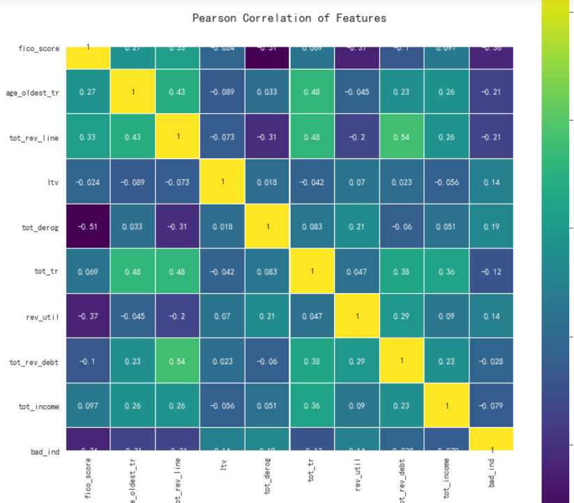
#用热力图看看相关性
colormap = plt.cm.viridis
plt.figure(figsize=(12,12))
plt.title(‘Pearson Correlation of Features‘, y=1.05, size=15)
sns.heatmap(df.corr(),linewidths=0.1,vmax=1.0, square=True, cmap=colormap, linecolor=‘white‘, annot=True)
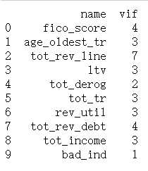
#利用VIF(方差膨胀系数)检验多重共线性
from statsmodels.stats.outliers_influence import variance_inflation_factor as VIF
VIF_ls=[]
n=df.columns
for i in range(len(n)):
    VIF_ls.append([n[i],int(VIF(df.values,i))])
df_vif=pd.DataFrame(VIF_ls,columns=["name","vif"])
print(df_vif)
#利用协方差计算线性相关性
cor=df[col].corr()
cor.iloc[:,:]=np.tril(cor.values,k=-1)
cor=cor.stack()
cor[np.abs(cor)>0.7]
目前为止剩余变量不用处理,开始建模
# 用woe编码替换原属性值,这样可以让系数正则化
for i in range(len(x.columns)):
    x[x.columns[i]].replace(WOE[x.columns[i]],inplace=True)
x_list=list(df.columns)
x_list.remove("bad_ind")
x=df[x_list]
y=df["bad_ind"]
处理样本不平衡问题
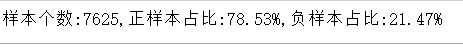
n_sample=y.shape[0]
n_pos_sample=y[y==0].shape[0]
n_neg_sample=y[y==1].shape[0]
print("样本个数:{},正样本占比:{:.2%},负样本占比:{:.2%}".format(n_sample,
                                         n_pos_sample/n_sample,
                                        n_neg_sample/n_sample))
from imblearn.over_sampling import SMOTE # 导入SMOTE算法模块
#from imblearn.over_sampling import BorderlineSMOTE
# 处理不平衡数据
sm = SMOTE(random_state=42)    # 处理过采样的方法
x_1, y_1 = sm.fit_sample(x, y)
print(‘通过SMOTE方法平衡正负样本后‘)
n_sample = y_1.shape[0]
n_pos_sample = y_1[y_1 == 0].shape[0]
n_neg_sample = y_1[y_1 == 1].shape[0]
print(‘样本个数:{}; 正样本占{:.2%}; 负样本占{:.2%}‘.format(n_sample,
                                                   n_pos_sample / n_sample,
                                                   n_neg_sample / n_sample))

#切分数据集与训练集
from sklearn.model_selection import train_test_split
X_train_1, X_test_1, y_train_1, y_test_1 = train_test_split(x_1,y_1,test_size = 0.3, random_state = 0)
X_train, X_test, y_train, y_test = train_test_split(x,y,test_size = 0.3, random_state = 0)
这里切分数据集一眼留作两份,实验在做样本均衡处理与不处理之间的差异
#逻辑回归训练并预测
import itertools
from sklearn.linear_model import LogisticRegression
from sklearn.metrics import confusion_matrix,recall_score,classification_report
lr = LogisticRegression(C = 1, penalty = ‘l2‘)
lr.fit(X_train_1,y_train_1.values.ravel())
y_pred = lr.predict(X_test_1.values)
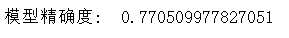
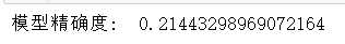
#计算混淆矩阵
from sklearn.metrics import confusion_matrix
cnf_matrix = confusion_matrix(y_test_1,y_pred)
np.set_printoptions(precision=2)
print("模型精确度: ", cnf_matrix[1,1]/(cnf_matrix[1,0]+cnf_matrix[1,1]))
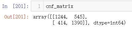
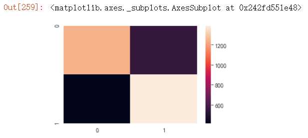
#绘制混淆矩阵
plt.figure(figsize=(5,3))
sns.heatmap(cnf_matrix)
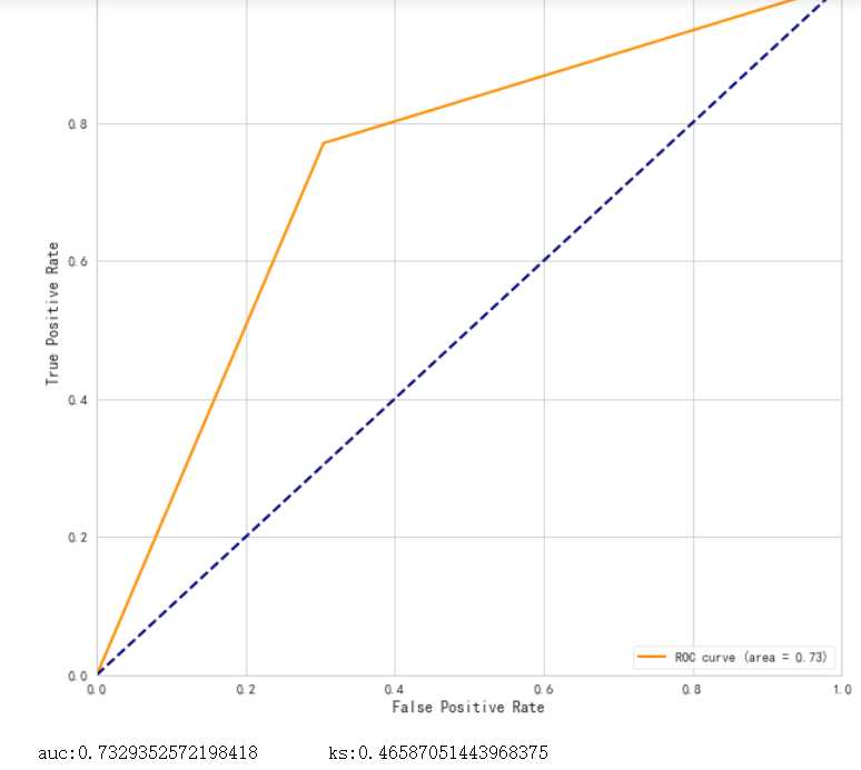
#绘制ROC曲线
from sklearn.metrics import roc_curve, auc
fpr,tpr,threshold = roc_curve(y_test_1,y_pred, drop_intermediate=False) ###计算真正率和假正率
roc_auc = auc(fpr,tpr) ###计算auc的值
ks=max(tpr-fpr)
plt.figure()
lw = 2
plt.figure(figsize=(10,10))
plt.plot(fpr, tpr, color=‘darkorange‘,
         lw=lw, label=‘ROC curve (area = %0.2f)‘ % roc_auc) ###假正率为横坐标,真正率为纵坐标做曲线
plt.plot([0, 1], [0, 1], color=‘navy‘, lw=lw, linestyle=‘--‘)
plt.xlim([0.0, 1.0])
plt.ylim([0.0, 1.05])
plt.xlabel(‘False Positive Rate‘)
plt.ylabel(‘True Positive Rate‘)
plt.title("ROC 曲线")
plt.legend(loc="lower right")
plt.show()
print("auc:{}       ks:{}".format(roc_auc,ks))
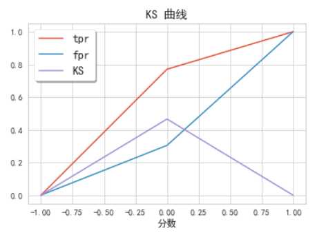
# 利用sklearn.metrics中的roc_curve算出tpr,fpr作图


fig, ax = plt.subplots()
ax.plot(1 - threshold, tpr, label=‘tpr‘) # ks曲线要按照预测概率降序排列,所以需要1-threshold镜像
ax.plot(1 - threshold, fpr, label=‘fpr‘)
ax.plot(1 - threshold, tpr-fpr,label=‘KS‘)
plt.xlabel(‘分数‘)
plt.title(‘KS 曲线‘)
#plt.xticks(np.arange(0,1,0.2), np.arange(1,0,-0.2))
#plt.xticks(np.arange(0,1,0.2), np.arange(score.max(),score.min(),-0.2*(data[‘反欺诈评分卡总分‘].max() - data[‘反欺诈评分卡总分‘].min())))
plt.figure(figsize=(20,20))
legend = ax.legend(loc=‘upper left‘, shadow=True, fontsize=‘x-large‘)

plt.show()
coef=lr.coef_#模型输出系数
intercept=lr.intercept_#模型输出截距
#变量集v与对应系数coef组合:v_coef
df_v=pd.DataFrame(col)
df_coef=pd.DataFrame(coef.T,index=col)

#v_coef=pd.concat([df_v,df_coef],axis=1)
#v_coef.columns=[‘var_name‘,‘coef‘]
#v_coef
df_coef.T
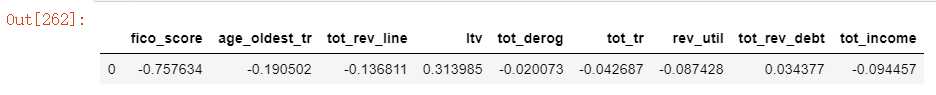
intercept
#输出评分卡
#假设比率为1/20 时 分值是500,比率每翻倍一次的20分
B=20/np.log(2)
A=500+B*np.log(1/20)
basescore=round(A-B*1.63,0) #基准分四舍五入取
scores=woe0*B
for i in col:
    scores[i]=scores[i].apply(lambda x:-round(x*df_coef.T[i],0))
print("基准分等于","\t",basescore)
print("各项得分等于")
scores
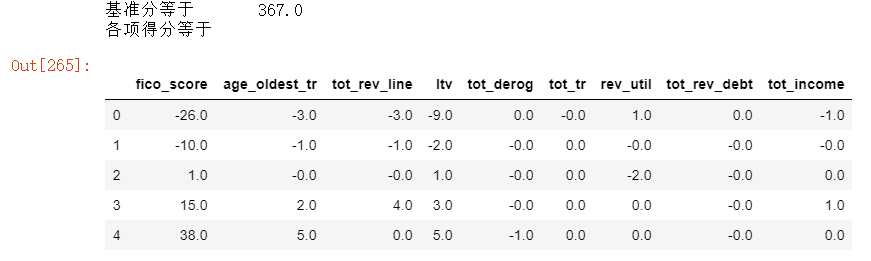
以上为分箱最小箱比列为0 ,且经过样本平衡处理的结果
之后分别计算了不同参数下的结果
1.以上为分箱最小箱比列为0 ,未作样本平衡处理结果
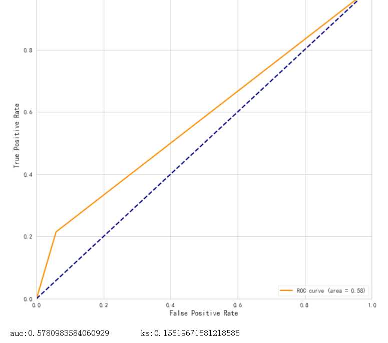
结果很差,可能是因为样本数据较小,所以样本平衡显得尤其重要
2.分箱最小箱比列为0 ,且经过样本平衡处理的结果,经过单调性检验并合并分箱之后的结果

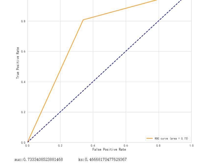
精确度有所提升,但是模型效力提升效果不显著
之后的样本建模任然没有太大变化。
总结:
1.分箱方案的选择,可能直接影响到特征的选择,所以需要多尝试几次,尽量选择最优的方案
2.模型的建立,本身是一个所有步骤不断迭代的过程,从缺失值填充开始,就需要不断的尝试不同方案,用来提升模型效力
还缺少一个完整的评分卡展示。。。。后面再补上
标签:actor fonts 不执行 enumerate point 缺失值 statistic reset 坐标
原文地址:https://www.cnblogs.com/Koi504330/p/12333807.html
