标签:rdb weight 预测 info tin read mod format knn
目录
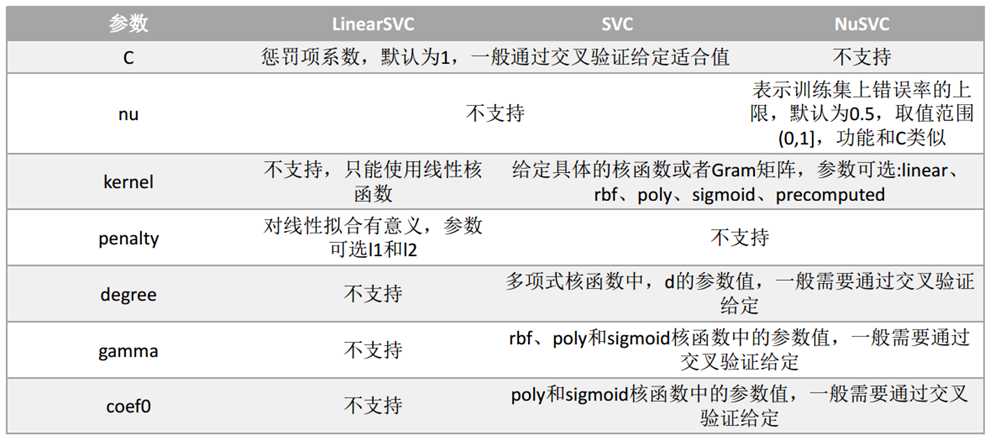
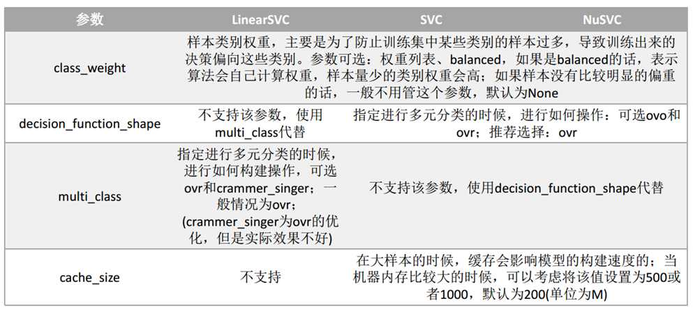
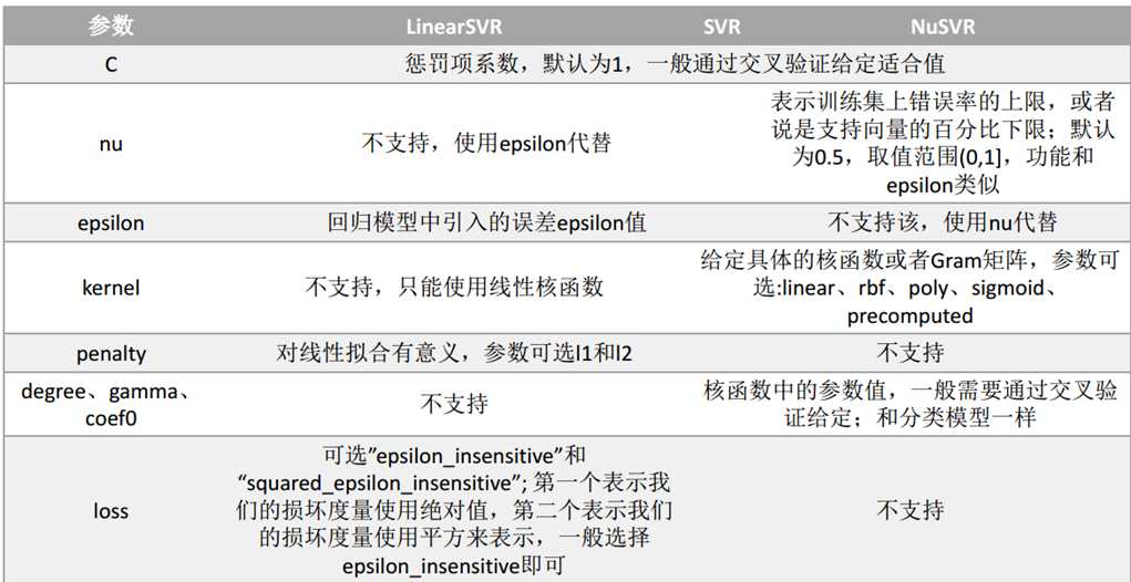
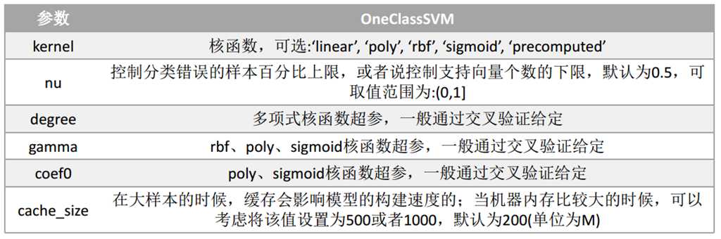
svm.SVC API说明:也可见另一篇博文:https://www.cnblogs.com/yifanrensheng/p/11863324.html
参数说明:
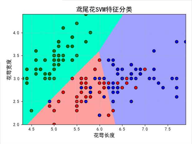
1 2 3 4 5 6 7 8 9 10 11 12 13 14 15 16 17 18 19 20 21 22 23 24 25 26 27 28 29 30 31 32 33 34 35 36 37 38 39 40 41 42 43 44 45 46 47 48 49 50 51 52 53 54 55 56 57 58 59 60 61 62 63 64 65 66 67 68 69 70 71 72 73 74 75 76 | # Author:yifan import numpy as np import pandas as pd import matplotlib as mpl import matplotlib.pyplot as plt import warnings ? ? from sklearn import svm #svm导入 from sklearn.model_selection import train_test_split from sklearn.metrics import accuracy_score from sklearn.exceptions import ChangedBehaviorWarning ? ? ## 设置属性防止中文乱码 mpl.rcParams[‘font.sans-serif‘] = [u‘SimHei‘] mpl.rcParams[‘axes.unicode_minus‘] = False ? ? warnings.filterwarnings(‘ignore‘, category=ChangedBehaviorWarning) ? ? ## 读取数据 # ‘sepal length‘, ‘sepal width‘, ‘petal length‘, ‘petal width‘ iris_feature = u‘花萼长度‘, u‘花萼宽度‘, u‘花瓣长度‘, u‘花瓣宽度‘ path = ‘./datas/iris.data‘ # 数据文件路径 data = pd.read_csv(path, header=None) x, y = data[list(range(4))], data[4] y = pd.Categorical(y).codes #把文本数据进行编码,比如a b c编码为 0 1 2; 可以通过pd.Categorical(y).categories获取index对应的原始值 x = x[[0, 1]] # 获取第一列和第二列 ? ? ## 数据分割 x_train, x_test, y_train, y_test = train_test_split(x, y, random_state=0, train_size=0.8) ## 数据SVM分类器构建 clf = svm.SVC(C=1,kernel=‘rbf‘,gamma=0.1) #gamma值越大,训练集的拟合就越好,但是会造成过拟合,导致测试集拟合变差 #gamma值越小,模型的泛化能力越好,训练集和测试集的拟合相近,但是会导致训练集出现欠拟合问题,从而,准确率变低,导致测试集准确率也变低。 ## 模型训练 #SVC(C=1, cache_size=200, class_weight=None, coef0=0.0,decision_function_shape=None, degree=3, gamma=0.1, kernel=‘rbf‘, #max_iter=-1, probability=False, random_state=None, shrinking=True, tol=0.001, verbose=False) clf.fit(x_train, y_train) ? ? ## 计算模型的准确率/精度 print (clf.score(x_train, y_train)) print (‘训练集准确率:‘, accuracy_score(y_train, clf.predict(x_train))) print (clf.score(x_test, y_test)) print (‘测试集准确率:‘, accuracy_score(y_test, clf.predict(x_test))) ? ? # 画图 N = 500 x1_min, x2_min = x.min() x1_max, x2_max = x.max() # print(x.max()) t1 = np.linspace(x1_min, x1_max, N) t2 = np.linspace(x2_min, x2_max, N) x1, x2 = np.meshgrid(t1, t2) # 生成网格采样点 grid_show = np.dstack((x1.flat, x2.flat))[0] # 测试点 ? ? grid_hat = clf.predict(grid_show) # 预测分类值 grid_hat = grid_hat.reshape(x1.shape) # 使之与输入的形状相同 ? ? cm_light = mpl.colors.ListedColormap([‘#00FFCC‘, ‘#FFA0A0‘, ‘#A0A0FF‘]) cm_dark = mpl.colors.ListedColormap([‘g‘, ‘r‘, ‘b‘]) plt.figure(facecolor=‘w‘) ## 区域图 plt.pcolormesh(x1, x2, grid_hat, cmap=cm_light) ## 所以样本点 plt.scatter(x[0], x[1], c=y, edgecolors=‘k‘, s=50, cmap=cm_dark) # 样本 ## 测试数据集 plt.scatter(x_test[0], x_test[1], s=120, facecolors=‘none‘, zorder=10) # 圈中测试集样本 ## lable列表 plt.xlabel(iris_feature[0], fontsize=13) plt.ylabel(iris_feature[1], fontsize=13) plt.xlim(x1_min, x1_max) plt.ylim(x2_min, x2_max) plt.title(u‘鸢尾花SVM特征分类‘, fontsize=16) plt.grid(b=True, ls=‘:‘) plt.tight_layout(pad=1.5) plt.show() |
0.85
训练集准确率: 0.85
0.7333333333333333
测试集准确率: 0.7333333333333333
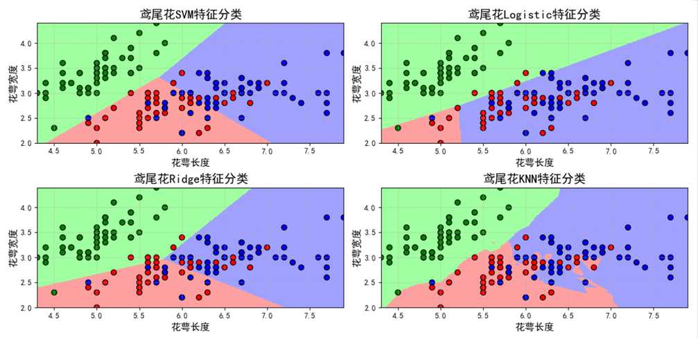
1 2 3 4 5 6 7 8 9 10 11 12 13 14 15 16 17 18 19 20 21 22 23 24 25 26 27 28 29 30 31 32 33 34 35 36 37 38 39 40 41 42 43 44 45 46 47 48 49 50 51 52 53 54 55 56 57 58 59 60 61 62 63 64 65 66 67 68 69 70 71 72 73 74 75 76 77 78 79 80 81 82 83 84 85 86 87 88 89 90 91 92 93 94 95 96 97 98 99 100 101 102 103 104 105 106 107 108 109 110 111 112 113 114 115 116 117 118 119 120 121 122 123 124 125 126 127 128 129 130 131 132 133 134 135 136 137 138 139 140 141 142 143 144 145 146 147 148 149 150 151 152 153 154 155 156 157 158 159 160 161 162 163 164 | # Author:yifan ? ? import numpy as np import pandas as pd import matplotlib as mpl import matplotlib.pyplot as plt from sklearn.svm import SVC from sklearn.model_selection import train_test_split from sklearn.metrics import accuracy_score from sklearn.linear_model import LogisticRegression,RidgeClassifier from sklearn.neighbors import KNeighborsClassifier ? ? ## 设置属性防止中文乱码 mpl.rcParams[‘font.sans-serif‘] = [u‘SimHei‘] mpl.rcParams[‘axes.unicode_minus‘] = False ## 读取数据 # ‘sepal length‘, ‘sepal width‘, ‘petal length‘, ‘petal width‘ iris_feature = u‘花萼长度‘, u‘花萼宽度‘, u‘花瓣长度‘, u‘花瓣宽度‘ path = ‘./datas/iris.data‘ # 数据文件路径 data = pd.read_csv(path, header=None) x, y = data[list(range(4))], data[4] y = pd.Categorical(y).codes x = x[[0, 1]] ? ? ## 数据分割 x_train, x_test, y_train, y_test = train_test_split(x, y, random_state=28, train_size=0.6) ? ? # 数据SVM分类器构建 svm = SVC(C=1, kernel=‘linear‘) ## Linear分类器构建 lr = LogisticRegression() rc = RidgeClassifier()#ridge是为了解决特征大于样本,而导致分类效果较差的情况,而提出的 #svm有一个重要的瓶颈——当特征数大于样本数的时候,效果变差 knn = KNeighborsClassifier() ? ? ## 模型训练 svm.fit(x_train, y_train) lr.fit(x_train, y_train) rc.fit(x_train, y_train) knn.fit(x_train, y_train) ? ? ## 效果评估 svm_score1 = accuracy_score(y_train, svm.predict(x_train)) svm_score2 = accuracy_score(y_test, svm.predict(x_test)) ? ? lr_score1 = accuracy_score(y_train, lr.predict(x_train)) lr_score2 = accuracy_score(y_test, lr.predict(x_test)) ? ? rc_score1 = accuracy_score(y_train, rc.predict(x_train)) rc_score2 = accuracy_score(y_test, rc.predict(x_test)) ? ? knn_score1 = accuracy_score(y_train, knn.predict(x_train)) knn_score2 = accuracy_score(y_test, knn.predict(x_test)) ? ? ## 画图 x_tmp = [0,1,2,3] y_score1 = [svm_score1, lr_score1, rc_score1, knn_score1] y_score2 = [svm_score2, lr_score2, rc_score2, knn_score2] ? ? plt.figure(facecolor=‘w‘) plt.plot(x_tmp, y_score1, ‘r-‘, lw=2, label=u‘训练集准确率‘) plt.plot(x_tmp, y_score2, ‘g-‘, lw=2, label=u‘测试集准确率‘) plt.xlim(0, 3) plt.ylim(np.min((np.min(y_score1), np.min(y_score2)))*0.9, np.max((np.max(y_score1), np.max(y_score2)))*1.1) plt.legend(loc = ‘lower right‘) plt.title(u‘鸢尾花数据不同分类器准确率比较‘, fontsize=16) plt.xticks(x_tmp, [u‘SVM‘, u‘Logistic‘, u‘Ridge‘, u‘KNN‘], rotation=0) plt.grid(b=True) plt.show() ? ? ? ? ### 画图比较 N = 500 x1_min, x2_min = x.min() x1_max, x2_max = x.max() ? ? t1 = np.linspace(x1_min, x1_max, N) t2 = np.linspace(x2_min, x2_max, N) x1, x2 = np.meshgrid(t1, t2) # 生成网格采样点 grid_show = np.dstack((x1.flat, x2.flat))[0] # 测试点 ? ? ## 获取各个不同算法的测试值 svm_grid_hat = svm.predict(grid_show) svm_grid_hat = svm_grid_hat.reshape(x1.shape) # 使之与输入的形状相同 ? ? lr_grid_hat = lr.predict(grid_show) lr_grid_hat = lr_grid_hat.reshape(x1.shape) # 使之与输入的形状相同 ? ? rc_grid_hat = rc.predict(grid_show) rc_grid_hat = rc_grid_hat.reshape(x1.shape) # 使之与输入的形状相同 ? ? knn_grid_hat = knn.predict(grid_show) knn_grid_hat = knn_grid_hat.reshape(x1.shape) # 使之与输入的形状相同 ? ? ## 画图 cm_light = mpl.colors.ListedColormap([‘#A0FFA0‘, ‘#FFA0A0‘, ‘#A0A0FF‘]) cm_dark = mpl.colors.ListedColormap([‘g‘, ‘r‘, ‘b‘]) plt.figure(facecolor=‘w‘, figsize=(14,7)) ? ? ### svm 区域图 plt.subplot(221) plt.pcolormesh(x1, x2, svm_grid_hat, cmap=cm_light) ## 所以样本点 plt.scatter(x[0], x[1], c=y, edgecolors=‘k‘, s=50, cmap=cm_dark) # 样本 ## 测试数据集 plt.scatter(x_test[0], x_test[1], s=120, facecolors=‘none‘, zorder=10) # 圈中测试集样本 ## lable列表 plt.xlabel(iris_feature[0], fontsize=13) plt.ylabel(iris_feature[1], fontsize=13) plt.xlim(x1_min, x1_max) plt.ylim(x2_min, x2_max) plt.title(u‘鸢尾花SVM特征分类‘, fontsize=16) plt.grid(b=True, ls=‘:‘) plt.tight_layout(pad=1.5) ? ? plt.subplot(222) ## 区域图 plt.pcolormesh(x1, x2, lr_grid_hat, cmap=cm_light) ## 所以样本点 plt.scatter(x[0], x[1], c=y, edgecolors=‘k‘, s=50, cmap=cm_dark) # 样本 ## 测试数据集 plt.scatter(x_test[0], x_test[1], s=120, facecolors=‘none‘, zorder=10) # 圈中测试集样本 ## lable列表 plt.xlabel(iris_feature[0], fontsize=13) plt.ylabel(iris_feature[1], fontsize=13) plt.xlim(x1_min, x1_max) plt.ylim(x2_min, x2_max) plt.title(u‘鸢尾花Logistic特征分类‘, fontsize=16) plt.grid(b=True, ls=‘:‘) plt.tight_layout(pad=1.5) ? ? plt.subplot(223) ## 区域图 plt.pcolormesh(x1, x2, rc_grid_hat, cmap=cm_light) ## 所以样本点 plt.scatter(x[0], x[1], c=y, edgecolors=‘k‘, s=50, cmap=cm_dark) # 样本 ## 测试数据集 plt.scatter(x_test[0], x_test[1], s=120, facecolors=‘none‘, zorder=10) # 圈中测试集样本 ## lable列表 plt.xlabel(iris_feature[0], fontsize=13) plt.ylabel(iris_feature[1], fontsize=13) plt.xlim(x1_min, x1_max) plt.ylim(x2_min, x2_max) plt.title(u‘鸢尾花Ridge特征分类‘, fontsize=16) plt.grid(b=True, ls=‘:‘) plt.tight_layout(pad=1.5) ? ? plt.subplot(224) ## 区域图 plt.pcolormesh(x1, x2, knn_grid_hat, cmap=cm_light) ## 所以样本点 plt.scatter(x[0], x[1], c=y, edgecolors=‘k‘, s=50, cmap=cm_dark) # 样本 ## 测试数据集 plt.scatter(x_test[0], x_test[1], s=120, facecolors=‘none‘, zorder=10) # 圈中测试集样本 ## lable列表 plt.xlabel(iris_feature[0], fontsize=13) plt.ylabel(iris_feature[1], fontsize=13) plt.xlim(x1_min, x1_max) plt.ylim(x2_min, x2_max) plt.title(u‘鸢尾花KNN特征分类‘, fontsize=16) plt.grid(b=True, ls=‘:‘) plt.tight_layout(pad=1.5) plt.show() |

? ?
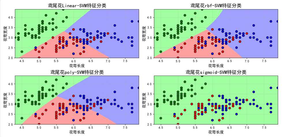
1 2 3 4 5 6 7 8 9 10 11 12 13 14 15 16 17 18 19 20 21 22 23 24 25 26 27 28 29 30 31 32 33 34 35 36 37 38 39 40 41 42 43 44 45 46 47 48 49 50 51 52 53 54 55 56 57 58 59 60 61 62 63 64 65 66 67 68 69 70 71 72 73 74 75 76 77 78 79 80 81 82 83 84 85 86 87 88 89 90 91 92 93 94 95 96 97 98 99 100 101 102 103 104 105 106 107 108 109 110 111 112 113 114 115 116 117 118 119 120 121 122 123 124 125 126 127 128 129 130 131 132 133 134 135 136 137 138 139 140 141 142 143 144 145 146 147 148 149 150 151 152 153 154 155 156 157 158 159 160 161 162 163 164 165 166 167 168 169 170 171 172 173 174 175 176 177 178 179 | # Author:yifan import time import numpy as np import pandas as pd import matplotlib as mpl import matplotlib.pyplot as plt from sklearn.svm import SVC from sklearn.model_selection import train_test_split from sklearn.metrics import accuracy_score ? ? ## 设置属性防止中文乱码 mpl.rcParams[‘font.sans-serif‘] = [u‘SimHei‘] mpl.rcParams[‘axes.unicode_minus‘] = False ## 读取数据 # ‘sepal length‘, ‘sepal width‘, ‘petal length‘, ‘petal width‘ iris_feature = u‘花萼长度‘, u‘花萼宽度‘, u‘花瓣长度‘, u‘花瓣宽度‘ path = ‘./datas/iris.data‘ # 数据文件路径 data = pd.read_csv(path, header=None) x, y = data[list(range(4))], data[4] y = pd.Categorical(y).codes x = x[[0, 1]] ? ? ## 数据分割 x_train, x_test, y_train, y_test = train_test_split(x, y, random_state=28, train_size=0.6) ? ? ## 数据SVM分类器构建 svm1 = SVC(C=1, kernel=‘linear‘) svm2 = SVC(C=1, kernel=‘rbf‘) svm3 = SVC(C=1, kernel=‘poly‘) svm4 = SVC(C=1, kernel=‘sigmoid‘) ? ? ## 模型训练 t0=time.time() svm1.fit(x_train, y_train) t1=time.time() svm2.fit(x_train, y_train) t2=time.time() svm3.fit(x_train, y_train) t3=time.time() svm4.fit(x_train, y_train) t4=time.time() ? ? ### 效果评估 svm1_score1 = accuracy_score(y_train, svm1.predict(x_train)) svm1_score2 = accuracy_score(y_test, svm1.predict(x_test)) ? ? svm2_score1 = accuracy_score(y_train, svm2.predict(x_train)) svm2_score2 = accuracy_score(y_test, svm2.predict(x_test)) ? ? svm3_score1 = accuracy_score(y_train, svm3.predict(x_train)) svm3_score2 = accuracy_score(y_test, svm3.predict(x_test)) ? ? svm4_score1 = accuracy_score(y_train, svm4.predict(x_train)) svm4_score2 = accuracy_score(y_test, svm4.predict(x_test)) ? ? ## 画图 x_tmp = [0,1,2,3] t_score = [t1 - t0, t2-t1, t3-t2, t4-t3] y_score1 = [svm1_score1, svm2_score1, svm3_score1, svm4_score1] y_score2 = [svm1_score2, svm2_score2, svm3_score2, svm4_score2] ? ? plt.figure(facecolor=‘w‘, figsize=(12,6)) ? ? ? ? plt.subplot(121) plt.plot(x_tmp, y_score1, ‘r-‘, lw=2, label=u‘训练集准确率‘) plt.plot(x_tmp, y_score2, ‘g-‘, lw=2, label=u‘测试集准确率‘) plt.xlim(-0.3, 3.3) plt.ylim(np.min((np.min(y_score1), np.min(y_score2)))*0.9, np.max((np.max(y_score1), np.max(y_score2)))*1.1) plt.legend(loc = ‘lower left‘) plt.title(u‘模型预测准确率‘, fontsize=13) plt.xticks(x_tmp, [u‘linear-SVM‘, u‘rbf-SVM‘, u‘poly-SVM‘, u‘sigmoid-SVM‘], rotation=0) plt.grid(b=True) ? ? plt.subplot(122) plt.plot(x_tmp, t_score, ‘b-‘, lw=2, label=u‘模型训练时间‘) plt.title(u‘模型训练耗时‘, fontsize=13) plt.xticks(x_tmp, [u‘linear-SVM‘, u‘rbf-SVM‘, u‘poly-SVM‘, u‘sigmoid-SVM‘], rotation=0) plt.xlim(-0.3, 3.3) plt.grid(b=True) plt.suptitle(u‘鸢尾花数据SVM分类器不同内核函数模型比较‘, fontsize=16) ? ? plt.show() ? ? ? ? ### 预测结果画图 ### 画图比较 N = 500 x1_min, x2_min = x.min() x1_max, x2_max = x.max() ? ? t1 = np.linspace(x1_min, x1_max, N) t2 = np.linspace(x2_min, x2_max, N) x1, x2 = np.meshgrid(t1, t2) # 生成网格采样点 grid_show = np.dstack((x1.flat, x2.flat))[0] # 测试点 ? ? ## 获取各个不同算法的测试值 svm1_grid_hat = svm1.predict(grid_show) svm1_grid_hat = svm1_grid_hat.reshape(x1.shape) # 使之与输入的形状相同 ? ? svm2_grid_hat = svm2.predict(grid_show) svm2_grid_hat = svm2_grid_hat.reshape(x1.shape) # 使之与输入的形状相同 ? ? svm3_grid_hat = svm3.predict(grid_show) svm3_grid_hat = svm3_grid_hat.reshape(x1.shape) # 使之与输入的形状相同 ? ? svm4_grid_hat = svm4.predict(grid_show) svm4_grid_hat = svm4_grid_hat.reshape(x1.shape) # 使之与输入的形状相同 ? ? ## 画图 cm_light = mpl.colors.ListedColormap([‘#A0FFA0‘, ‘#FFA0A0‘, ‘#A0A0FF‘]) cm_dark = mpl.colors.ListedColormap([‘g‘, ‘r‘, ‘b‘]) plt.figure(facecolor=‘w‘, figsize=(14,7)) ? ? ### svm plt.subplot(221) ## 区域图 plt.pcolormesh(x1, x2, svm1_grid_hat, cmap=cm_light) ## 所以样本点 plt.scatter(x[0], x[1], c=y, edgecolors=‘k‘, s=50, cmap=cm_dark) # 样本 ## 测试数据集 plt.scatter(x_test[0], x_test[1], s=120, facecolors=‘none‘, zorder=10) # 圈中测试集样本 ## lable列表 plt.xlabel(iris_feature[0], fontsize=13) plt.ylabel(iris_feature[1], fontsize=13) plt.xlim(x1_min, x1_max) plt.ylim(x2_min, x2_max) plt.title(u‘鸢尾花Linear-SVM特征分类‘, fontsize=16) plt.grid(b=True, ls=‘:‘) plt.tight_layout(pad=1.5) ? ? plt.subplot(222) ## 区域图 plt.pcolormesh(x1, x2, svm2_grid_hat, cmap=cm_light) ## 所以样本点 plt.scatter(x[0], x[1], c=y, edgecolors=‘k‘, s=50, cmap=cm_dark) # 样本 ## 测试数据集 plt.scatter(x_test[0], x_test[1], s=120, facecolors=‘none‘, zorder=10) # 圈中测试集样本 ## lable列表 plt.xlabel(iris_feature[0], fontsize=13) plt.ylabel(iris_feature[1], fontsize=13) plt.xlim(x1_min, x1_max) plt.ylim(x2_min, x2_max) plt.title(u‘鸢尾花rbf-SVM特征分类‘, fontsize=16) plt.grid(b=True, ls=‘:‘) plt.tight_layout(pad=1.5) ? ? plt.subplot(223) ## 区域图 plt.pcolormesh(x1, x2, svm3_grid_hat, cmap=cm_light) ## 所以样本点 plt.scatter(x[0], x[1], c=y, edgecolors=‘k‘, s=50, cmap=cm_dark) # 样本 ## 测试数据集 plt.scatter(x_test[0], x_test[1], s=120, facecolors=‘none‘, zorder=10) # 圈中测试集样本 ## lable列表 plt.xlabel(iris_feature[0], fontsize=13) plt.ylabel(iris_feature[1], fontsize=13) plt.xlim(x1_min, x1_max) plt.ylim(x2_min, x2_max) plt.title(u‘鸢尾花poly-SVM特征分类‘, fontsize=16) plt.grid(b=True, ls=‘:‘) plt.tight_layout(pad=1.5) ? ? plt.subplot(224) ## 区域图 plt.pcolormesh(x1, x2, svm4_grid_hat, cmap=cm_light) ## 所以样本点 plt.scatter(x[0], x[1], c=y, edgecolors=‘k‘, s=50, cmap=cm_dark) # 样本 ## 测试数据集 plt.scatter(x_test[0], x_test[1], s=120, facecolors=‘none‘, zorder=10) # 圈中测试集样本 ## lable列表 plt.xlabel(iris_feature[0], fontsize=13) plt.ylabel(iris_feature[1], fontsize=13) plt.xlim(x1_min, x1_max) plt.ylim(x2_min, x2_max) plt.title(u‘鸢尾花sigmoid-SVM特征分类‘, fontsize=16) plt.grid(b=True, ls=‘:‘) plt.tight_layout(pad=1.5) plt.show() |

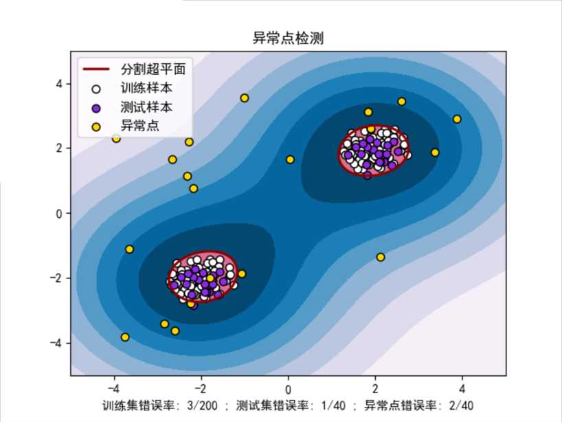
1 2 3 4 5 6 7 8 9 10 11 12 13 14 15 16 17 18 19 20 21 22 23 24 25 26 27 28 29 30 31 32 33 34 35 36 37 38 39 40 41 42 43 44 45 46 47 48 49 50 51 52 53 54 55 56 57 58 59 60 61 62 63 | # Author:yifan import numpy as np import matplotlib.pyplot as plt import matplotlib as mpl import matplotlib.font_manager from sklearn import svm ## 设置属性防止中文乱码 mpl.rcParams[‘font.sans-serif‘] = [u‘SimHei‘] mpl.rcParams[‘axes.unicode_minus‘] = False ? ? # 模拟数据产生 xx, yy = np.meshgrid(np.linspace(-5, 5, 500), np.linspace(-5, 5, 500)) # 产生训练数据 X = 0.3 * np.random.randn(100, 2) X_train = np.r_[X + 2, X - 2] # 产测试数据 X = 0.3 * np.random.randn(20, 2) X_test = np.r_[X + 2, X - 2] # 产生一些异常点数据 X_outliers = np.random.uniform(low=-4, high=4, size=(20, 2)) ? ? # 模型训练 clf = svm.OneClassSVM(nu=0.01, kernel="rbf", gamma=0.1) clf.fit(X_train) ? ? # 预测结果获取 y_pred_train = clf.predict(X_train) y_pred_test = clf.predict(X_test) y_pred_outliers = clf.predict(X_outliers) # 返回1表示属于这个类别,-1表示不属于这个类别 n_error_train = y_pred_train[y_pred_train == -1].size n_error_test = y_pred_test[y_pred_test == -1].size n_error_outliers = y_pred_outliers[y_pred_outliers == 1].size ? ? # 获取绘图的点信息 Z = clf.decision_function(np.c_[xx.ravel(), yy.ravel()]) Z = Z.reshape(xx.shape) ? ? # 画图 plt.figure(facecolor=‘w‘) plt.title("异常点检测") # 画出区域图 plt.contourf(xx, yy, Z, levels=np.linspace(Z.min(), 0, 9), cmap=plt.cm.PuBu) a = plt.contour(xx, yy, Z, levels=[0], linewidths=2, colors=‘darkred‘) plt.contourf(xx, yy, Z, levels=[0, Z.max()], colors=‘palevioletred‘) # 画出点图 s = 40 b1 = plt.scatter(X_train[:, 0], X_train[:, 1], c=‘white‘, s=s, edgecolors=‘k‘) b2 = plt.scatter(X_test[:, 0], X_test[:, 1], c=‘blueviolet‘, s=s, edgecolors=‘k‘) c = plt.scatter(X_outliers[:, 0], X_outliers[:, 1], c=‘gold‘, s=s, edgecolors=‘k‘) ? ? # 设置相关信息 plt.axis(‘tight‘) plt.xlim((-5, 5)) plt.ylim((-5, 5)) plt.legend([a.collections[0], b1, b2, c], ["分割超平面", "训练样本", "测试样本", "异常点"], loc="upper left", prop=matplotlib.font_manager.FontProperties(size=11)) plt.xlabel("训练集错误率: %d/200 ; 测试集错误率: %d/40 ; 异常点错误率: %d/40" \ % (n_error_train, n_error_test, n_error_outliers)) plt.show() |
结果:
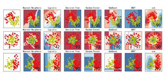
比较逻辑回归、KNN、决策树、随机森林、GBDT、Adaboost、SVM等分类算法的效果,数据集使用sklearn自带的模拟数据进行测试。
1 2 3 4 5 6 7 8 9 10 11 12 13 14 15 16 17 18 19 20 21 22 23 24 25 26 27 28 29 30 31 32 33 34 35 36 37 38 39 40 41 42 43 44 45 46 47 48 49 50 51 52 53 54 55 56 57 58 59 60 61 62 63 64 65 66 67 68 69 70 71 72 73 74 75 76 77 78 79 80 81 82 83 84 85 86 87 88 89 | # Author:yifan import numpy as np import matplotlib.pyplot as plt import matplotlib as mpl from matplotlib.colors import ListedColormap from sklearn import svm from sklearn.model_selection import train_test_split from sklearn.preprocessing import StandardScaler from sklearn.datasets import make_moons, make_circles, make_classification from sklearn.neighbors import KNeighborsClassifier from sklearn.tree import DecisionTreeClassifier from sklearn.ensemble import RandomForestClassifier, AdaBoostClassifier, GradientBoostingClassifier from sklearn.linear_model import LogisticRegressionCV ## 设置属性防止中文乱码 mpl.rcParams[‘font.sans-serif‘] = [u‘SimHei‘] mpl.rcParams[‘axes.unicode_minus‘] = False #构造数据 X, y = make_classification(n_features=2, n_redundant=0, n_informative=2,random_state=1, n_clusters_per_class=1) rng = np.random.RandomState(2) X += 2 * rng.uniform(size=X.shape) linearly_separable = (X, y) datasets = [make_moons(noise=0.3, random_state=0), make_circles(noise=0.2, factor=0.4, random_state=1), linearly_separable] #建模环节,用list把所有算法装起来 names = ["Nearest Neighbors", "Logistic","Decision Tree", "Random Forest", "AdaBoost", "GBDT","svm"] classifiers = [ KNeighborsClassifier(3), LogisticRegressionCV(), DecisionTreeClassifier(max_depth=5), RandomForestClassifier(max_depth=5, n_estimators=10, max_features=1), AdaBoostClassifier(n_estimators=10,learning_rate=1.5), GradientBoostingClassifier(n_estimators=10, learning_rate=1.5), svm.SVC(C=1, kernel=‘rbf‘) ] ## 画图 figure = plt.figure(figsize=(27, 9), facecolor=‘w‘) i = 1 h = .02 # 步长 ? ? for ds in datasets: X, y = ds X = StandardScaler().fit_transform(X) X_train, X_test, y_train, y_test = train_test_split(X, y, test_size=.4) x_min, x_max = X[:, 0].min() - .5, X[:, 0].max() + .5 y_min, y_max = X[:, 1].min() - .5, X[:, 1].max() + .5 xx, yy = np.meshgrid(np.arange(x_min, x_max, h), np.arange(y_min, y_max, h)) cm = plt.cm.RdBu cm_bright = ListedColormap([‘r‘, ‘b‘, ‘y‘]) ax = plt.subplot(len(datasets), len(classifiers) + 1, i) ax.scatter(X_train[:, 0], X_train[:, 1], c=y_train, cmap=cm_bright) ax.scatter(X_test[:, 0], X_test[:, 1], c=y_test, cmap=cm_bright, alpha=0.6) ax.set_xlim(xx.min(), xx.max()) ax.set_ylim(yy.min(), yy.max()) ax.set_xticks(()) ax.set_yticks(()) i += 1 # 画每个算法的图 for name, clf in zip(names, classifiers): ax = plt.subplot(len(datasets), len(classifiers) + 1, i) clf.fit(X_train, y_train) score = clf.score(X_test, y_test) # hasattr是判定某个模型中,有没有哪个参数, # 判断clf模型中,有没有decision_function # np.c_让内部数据按列合并 if hasattr(clf, "decision_function"): Z = clf.decision_function(np.c_[xx.ravel(), yy.ravel()]) else: Z = clf.predict_proba(np.c_[xx.ravel(), yy.ravel()])[:, 1] ? ? Z = Z.reshape(xx.shape) ax.contourf(xx, yy, Z, cmap=cm, alpha=.8) ax.scatter(X_train[:, 0], X_train[:, 1], c=y_train, cmap=cm_bright) ax.scatter(X_test[:, 0], X_test[:, 1], c=y_test, cmap=cm_bright, alpha=0.6) ? ? ax.set_xlim(xx.min(), xx.max()) ax.set_ylim(yy.min(), yy.max()) ax.set_xticks(()) ax.set_yticks(()) ax.set_title(name) ax.text(xx.max() - .3, yy.min() + .3, (‘%.2f‘ % score).lstrip(‘0‘), size=25, horizontalalignment=‘right‘) i += 1 ## 展示图 figure.subplots_adjust(left=.02, right=.98) plt.show() # plt.savefig("cs.png") |
结果:
? ?
? ?
? ?
【ML-9】支持向量机--实验scitit-learn SVM
标签:rdb weight 预测 info tin read mod format knn
原文地址:https://www.cnblogs.com/yifanrensheng/p/12354995.html