标签:obj arc body anova 控制 位置 功能 穷举 通过
本文主要内容摘自 易悠 博主的 Pima印第安人数据集上的机器学习-分类算法(根据诊断措施预测糖尿病的发病)
https://blog.csdn.net/yizheyouye/article/details/79791473
在一些地方做了补充说明,便于小白理解。
该数据集最初来自国家糖尿病/消化/肾脏疾病研究所。
数据集的目标是基于数据集中包含的某些诊断测量来诊断性的预测 患者是否患有糖尿病。
从较大的数据库中选择这些实例有几个约束条件。尤其是,这里的所有患者都是Pima印第安至少21岁的女性。
数据集由多个医学预测变量和一个目标变量组成Outcome。预测变量包括患者的怀孕次数、BMI、胰岛素水平、年龄等。
import xgboost as xgb
from sklearn.metrics import accuracy_score
from sklearn.feature_selection import SelectKBest
from sklearn.feature_selection import chi2
import pandas as pd
import matplotlib.pyplot as plt
import numpy as np
import seaborn as sns # matplotlib的高级API
from sklearn.preprocessing import StandardScaler #导入标准化功能
from sklearn.model_selection import train_test_split #构建二分类算法模型
pima = pd.read_csv("D:\\xgbtest\\pima-indians-diabetes.csv") pima.shape # panda的shape形状属性,给出对象的尺寸(行数目,列数目)(768, 9)# 查看Series或者DataFrame对象的小样本;显示的默认元素数量的前五个。可以自定义数量。
pima.head() | Pregnancies | Glucose | BloodPressure | SkinThickness | Insulin | BMI | DiabetesPedigreeFunction | Age | Outcome | |
|---|---|---|---|---|---|---|---|---|---|
| 0 | 6 | 148 | 72 | 35 | 0 | 33.6 | 0.627 | 50 | 1 |
| 1 | 1 | 85 | 66 | 29 | 0 | 26.6 | 0.351 | 31 | 0 |
| 2 | 8 | 183 | 64 | 0 | 0 | 23.3 | 0.672 | 32 | 1 |
| 3 | 1 | 89 | 66 | 23 | 94 | 28.1 | 0.167 | 21 | 0 |
| 4 | 0 | 137 | 40 | 35 | 168 | 43.1 | 2.288 | 33 | 1 |
# panda的describe描述属性,展示了每一个字段的
#【count条目统计,mean平均值,std标准值,min最小值,25%,50%中位数,75%,max最大值】
pima.describe()| Pregnancies | Glucose | BloodPressure | SkinThickness | Insulin | BMI | DiabetesPedigreeFunction | Age | Outcome | |
|---|---|---|---|---|---|---|---|---|---|
| count | 768.000000 | 768.000000 | 768.000000 | 768.000000 | 768.000000 | 768.000000 | 768.000000 | 768.000000 | 768.000000 |
| mean | 3.845052 | 120.894531 | 69.105469 | 20.536458 | 79.799479 | 31.992578 | 0.471876 | 33.240885 | 0.348958 |
| std | 3.369578 | 31.972618 | 19.355807 | 15.952218 | 115.244002 | 7.884160 | 0.331329 | 11.760232 | 0.476951 |
| min | 0.000000 | 0.000000 | 0.000000 | 0.000000 | 0.000000 | 0.000000 | 0.078000 | 21.000000 | 0.000000 |
| 25% | 1.000000 | 99.000000 | 62.000000 | 0.000000 | 0.000000 | 27.300000 | 0.243750 | 24.000000 | 0.000000 |
| 50% | 3.000000 | 117.000000 | 72.000000 | 23.000000 | 30.500000 | 32.000000 | 0.372500 | 29.000000 | 0.000000 |
| 75% | 6.000000 | 140.250000 | 80.000000 | 32.000000 | 127.250000 | 36.600000 | 0.626250 | 41.000000 | 1.000000 |
| max | 17.000000 | 199.000000 | 122.000000 | 99.000000 | 846.000000 | 67.100000 | 2.420000 | 81.000000 | 1.000000 |
pima.groupby('Outcome').size() #将某Outcome分组统计Outcome
0 500
1 268
dtype: int64pima.hist(figsize=(16,14)) #查看每个字段的数据分布;figsize的参数显示的是每个子图的长和宽array([[<matplotlib.axes._subplots.AxesSubplot object at 0x000001F2B0715BC8>,
<matplotlib.axes._subplots.AxesSubplot object at 0x000001F2B09BBF88>,
<matplotlib.axes._subplots.AxesSubplot object at 0x000001F2B09FAF08>],
[<matplotlib.axes._subplots.AxesSubplot object at 0x000001F2B0A36048>,
<matplotlib.axes._subplots.AxesSubplot object at 0x000001F2B0A6C108>,
<matplotlib.axes._subplots.AxesSubplot object at 0x000001F2B0AA6208>],
[<matplotlib.axes._subplots.AxesSubplot object at 0x000001F2B0ADD308>,
<matplotlib.axes._subplots.AxesSubplot object at 0x000001F2B0B1DF48>,
<matplotlib.axes._subplots.AxesSubplot object at 0x000001F2B0B25048>]],
dtype=object)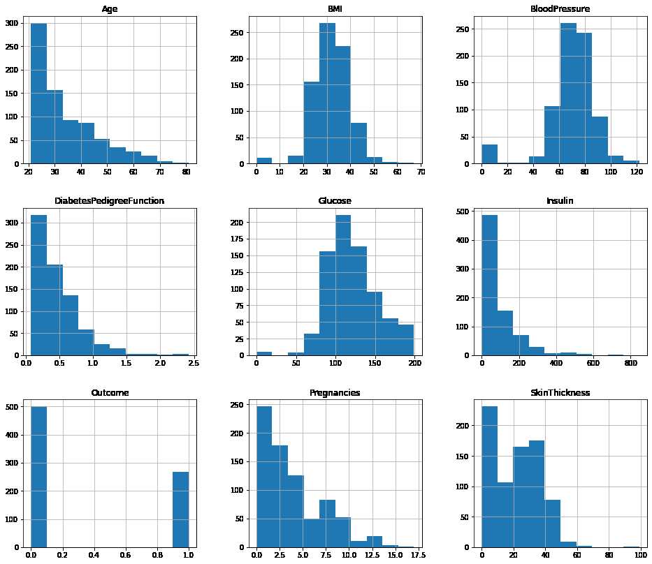
sns.pairplot(pima,hue='Outcome')
#对角线上是各个属性的直方图(分布图),而非对角线上是两个不同属性之间的相关图
# seaborn常用命令
#【1】set_style()是用来设置主题的,Seaborn有5个预设好的主题:darkgrid、whitegrid、dark、white、ticks,默认为darkgrid
#【2】set()通过设置参数可以用来设置背景,调色板等,更加常用
#【3】displot()为hist加强版
#【4】kdeplot()为密度曲线图
#【5】boxplot()为箱图
#【6】joinplot()联合分布图
#【7】heatmap()热点图
#【8】pairplot()多变量图,可以支持各种类型的变量分析,是特征分析很好用的工具
# hue :针对某一字段进行分类
# kind:用于控制非对角线上的图的类型,可选"scatter"与"reg"
C:\Anaconda3\lib\site-packages\statsmodels\nonparametric\kde.py:487: RuntimeWarning: invalid value encountered in true_divide
binned = fast_linbin(X, a, b, gridsize) / (delta * nobs)
C:\Anaconda3\lib\site-packages\statsmodels\nonparametric\kdetools.py:34: RuntimeWarning: invalid value encountered in double_scalars
FAC1 = 2*(np.pi*bw/RANGE)**2
<seaborn.axisgrid.PairGrid at 0x1f2b12b5e08>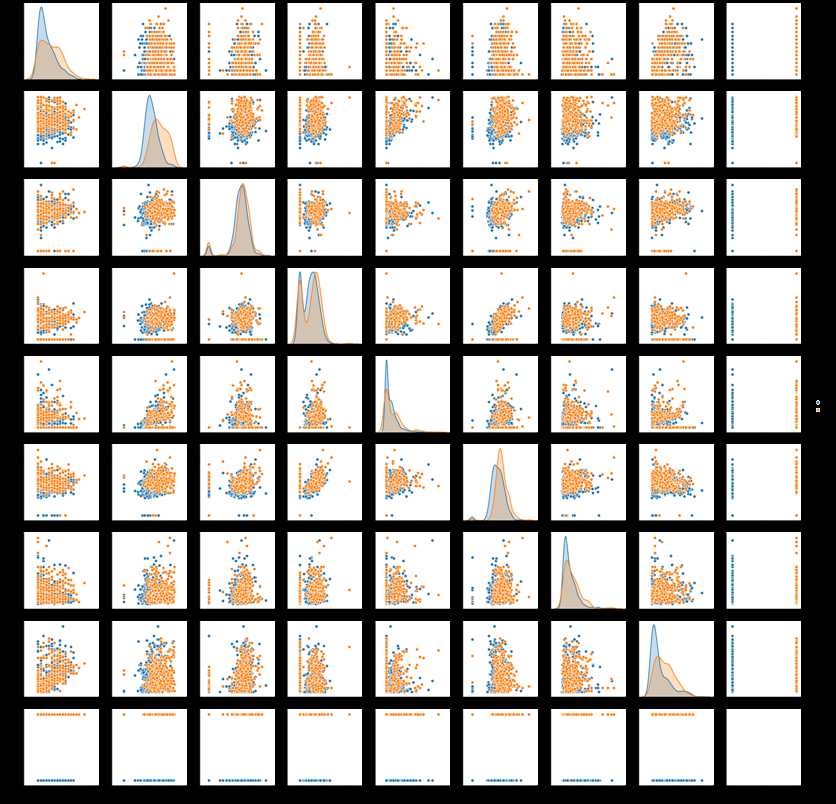
sns.pairplot(pima)<seaborn.axisgrid.PairGrid at 0x1f2b46b8908>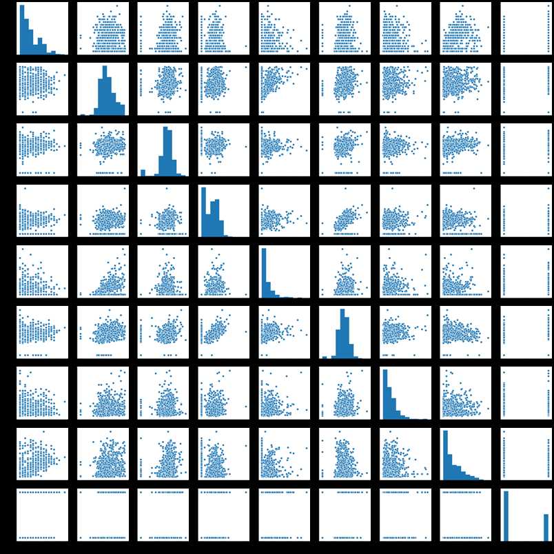
pima.plot(kind='box', subplots=True, layout=(3,3), sharex=False,sharey=False, figsize=(16,14))
#pandas.plot作图:数据分为Series 和 DataFrame两种类型;现释义数据为DataFrame的参数

#【0】data:DataFrame
#【1】x:label or position,default None 指数据框列的标签或位置参数
#【2】y:label or position,default None 指数据框列的标签或位置参数
#【3】kind:str(line折线图、bar条形图、barh横向条形图、hist柱状图、
#               box箱线图、kde Kernel的密度估计图,主要对柱状图添加Kernel概率密度线、
#               density same as “kde”、area区域图、pie饼图、scatter散点图、hexbin)
#【4】subplots:boolean,default False,为每一列单独画一个子图
#【5】sharex:boolean,default True if ax is None else False
#【6】sharey:boolean,default False
#【7】loglog:boolean,default False,x轴/y轴同时使用log刻度
Pregnancies AxesSubplot(0.125,0.657941;0.227941x0.222059)
Glucose AxesSubplot(0.398529,0.657941;0.227941x0.222059)
BloodPressure AxesSubplot(0.672059,0.657941;0.227941x0.222059)
SkinThickness AxesSubplot(0.125,0.391471;0.227941x0.222059)
Insulin AxesSubplot(0.398529,0.391471;0.227941x0.222059)
BMI AxesSubplot(0.672059,0.391471;0.227941x0.222059)
DiabetesPedigreeFunction AxesSubplot(0.125,0.125;0.227941x0.222059)
Age AxesSubplot(0.398529,0.125;0.227941x0.222059)
Outcome AxesSubplot(0.672059,0.125;0.227941x0.222059)
dtype: object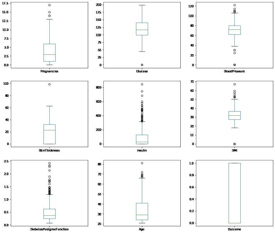
column_x = pima.columns[0:len(pima.columns) - 1] # 选择特征列,去掉目标列(Outcome)
column_x
Index(['Pregnancies', 'Glucose', 'BloodPressure', 'SkinThickness', 'Insulin',
'BMI', 'DiabetesPedigreeFunction', 'Age'],
dtype='object')corr = pima[pima.columns].corr() # 计算变量的相关系数,得到一个N * N的矩阵
corr| Pregnancies | Glucose | BloodPressure | SkinThickness | Insulin | BMI | DiabetesPedigreeFunction | Age | Outcome | |
|---|---|---|---|---|---|---|---|---|---|
| Pregnancies | 1.000000 | 0.129459 | 0.141282 | -0.081672 | -0.073535 | 0.017683 | -0.033523 | 0.544341 | 0.221898 |
| Glucose | 0.129459 | 1.000000 | 0.152590 | 0.057328 | 0.331357 | 0.221071 | 0.137337 | 0.263514 | 0.466581 |
| BloodPressure | 0.141282 | 0.152590 | 1.000000 | 0.207371 | 0.088933 | 0.281805 | 0.041265 | 0.239528 | 0.065068 |
| SkinThickness | -0.081672 | 0.057328 | 0.207371 | 1.000000 | 0.436783 | 0.392573 | 0.183928 | -0.113970 | 0.074752 |
| Insulin | -0.073535 | 0.331357 | 0.088933 | 0.436783 | 1.000000 | 0.197859 | 0.185071 | -0.042163 | 0.130548 |
| BMI | 0.017683 | 0.221071 | 0.281805 | 0.392573 | 0.197859 | 1.000000 | 0.140647 | 0.036242 | 0.292695 |
| DiabetesPedigreeFunction | -0.033523 | 0.137337 | 0.041265 | 0.183928 | 0.185071 | 0.140647 | 1.000000 | 0.033561 | 0.173844 |
| Age | 0.544341 | 0.263514 | 0.239528 | -0.113970 | -0.042163 | 0.036242 | 0.033561 | 1.000000 | 0.238356 |
| Outcome | 0.221898 | 0.466581 | 0.065068 | 0.074752 | 0.130548 | 0.292695 | 0.173844 | 0.238356 | 1.000000 |
plt.subplots(figsize=(10,5)) # 可以先试用plt设置画布的大小,然后在作图,修改
sns.heatmap(corr,annot = True) # 使用热度图可视化这个相关系数矩阵
<matplotlib.axes._subplots.AxesSubplot at 0x1f2bb97ab08>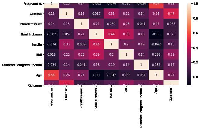
X=pima.iloc[:,0:8] #选取所有的行,选取前8列,不含Outcome
Y=pima.iloc[:,8] # 选出第9列。设为目标列
select_top_4=SelectKBest(score_func=chi2,k=4) # 通过卡方检验选择4个得分最高的特征fit = select_top_4.fit(X, Y) # 获取特征信息和目标值信息
features = fit.transform(X) # 特征转换
fit.get_support(indices=True).tolist() #得到宣传的相关性排名前4的列[1,4,5,7]
# 因此,表现最佳的特征是:Glucose-葡萄糖、Insulin-胰岛素、BMI指数、Age-年龄
# SelectKBest() 只保留K个最高分的特征
# SelectPercentile() 只保留用户指定百分比的最高得分的特征
# 使用常见的单变量统计检验:假正率SelectFpr,错误发现率SelectFdr,或者总体错误率SelectFwe
# GenericUnivariateSelect通过结构化策略进行特征选择,通过超参数搜索估计器进行特征选择
# SelectKBest()和SelectPercentile()能够返回特征评价的得分和P值
#
# sklearn.feature_selection.SelectPercentile(score_func=<function f_classif>, percentile=10)
# sklearn.feature_selection.SelectKBest(score_func=<function f_classif>, k=10)
# 其中的参数score_func有以下选项:
#【1】回归:f_regression:相关系数,计算每个变量与目标变量的相关系数,然后计算出F值和P值
# mutual_info_regression:互信息,互信息度量X和Y共享的信息:
# 它度量知道这两个变量其中一个,对另一个不确定度减少的程度。
#【2】分类:chi2:卡方检验
# f_classif:方差分析,计算方差分析(ANOVA)的F值(组间均方/组内均方);
# mutual_info_classif:互信息,互信息方法可以捕捉任何一种统计依赖,但是作为非参数方法,需要更多的样本进行准确的估计。[1, 4, 5, 7]features[0:5] #新特征列array([[148. , 0. , 33.6, 50. ],
[ 85. , 0. , 26.6, 31. ],
[183. , 0. , 23.3, 32. ],
[ 89. , 94. , 28.1, 21. ],
[137. , 168. , 43.1, 33. ]])pima.head()| Pregnancies | Glucose | BloodPressure | SkinThickness | Insulin | BMI | DiabetesPedigreeFunction | Age | Outcome | |
|---|---|---|---|---|---|---|---|---|---|
| 0 | 6 | 148 | 72 | 35 | 0 | 33.6 | 0.627 | 50 | 1 |
| 1 | 1 | 85 | 66 | 29 | 0 | 26.6 | 0.351 | 31 | 0 |
| 2 | 8 | 183 | 64 | 0 | 0 | 23.3 | 0.672 | 32 | 1 |
| 3 | 1 | 89 | 66 | 23 | 94 | 28.1 | 0.167 | 21 | 0 |
| 4 | 0 | 137 | 40 | 35 | 168 | 43.1 | 2.288 | 33 | 1 |
X_features = pd.DataFrame(data = features, columns=["Glucose","Insulin","BMI","Age"]) # 构造新特征DataFrameX_features.head()| Glucose | Insulin | BMI | Age | |
|---|---|---|---|---|
| 0 | 148.0 | 0.0 | 33.6 | 50.0 |
| 1 | 85.0 | 0.0 | 26.6 | 31.0 |
| 2 | 183.0 | 0.0 | 23.3 | 32.0 |
| 3 | 89.0 | 94.0 | 28.1 | 21.0 |
| 4 | 137.0 | 168.0 | 43.1 | 33.0 |
它将属性值更改为 均值为0,标准差为1 的 高斯分布.
当算法期望输入特征处于高斯分布时,它非常有用
rescaledX = StandardScaler().fit_transform(X_features) # 通过sklearn的preprocessing数据预处理中StandardScaler特征缩放 标准化特征信息X = pd.DataFrame(data = rescaledX, columns = X_features.columns) # 构建新特征DataFrameX.head()| Glucose | Insulin | BMI | Age | |
|---|---|---|---|---|
| 0 | 0.848324 | -0.692891 | 0.204013 | 1.425995 |
| 1 | -1.123396 | -0.692891 | -0.684422 | -0.190672 |
| 2 | 1.943724 | -0.692891 | -1.103255 | -0.105584 |
| 3 | -0.998208 | 0.123302 | -0.494043 | -1.041549 |
| 4 | 0.504055 | 0.765836 | 1.409746 | -0.020496 |
# 切分数据集为:特征训练集、特征测试集、目标训练集、目标测试集
X_train,X_test,Y_train,Y_test = train_test_split(X,Y, random_state = 22, test_size = 0.2) #test_size=0.2 表示测试集占20%。X_train.describe()| Glucose | Insulin | BMI | Age | |
|---|---|---|---|---|
| count | 614.000000 | 614.000000 | 614.000000 | 614.000000 |
| mean | 0.027972 | 0.026404 | -0.004205 | 0.013040 |
| std | 1.010934 | 1.044467 | 1.001749 | 1.000775 |
| min | -3.783654 | -0.692891 | -4.060474 | -1.041549 |
| 25% | -0.653939 | -0.692891 | -0.582887 | -0.786286 |
| 50% | -0.090591 | -0.380306 | 0.000942 | -0.360847 |
| 75% | 0.660541 | 0.435886 | 0.584771 | 0.638934 |
| max | 2.444478 | 6.652839 | 3.478529 | 4.063716 |
X_test.describe()| Glucose | Insulin | BMI | Age | |
|---|---|---|---|---|
| count | 154.000000 | 154.000000 | 154.000000 | 154.000000 |
| mean | -0.111523 | -0.105273 | 0.016766 | -0.051990 |
| std | 0.953583 | 0.796792 | 0.999346 | 1.001728 |
| min | -3.783654 | -0.692891 | -4.060474 | -1.041549 |
| 25% | -0.779128 | -0.692891 | -0.643173 | -0.871374 |
| 50% | -0.325319 | -0.692891 | 0.019980 | -0.445935 |
| 75% | 0.457109 | 0.303472 | 0.476889 | 0.660206 |
| max | 2.381884 | 3.474899 | 4.455807 | 2.787399 |
from sklearn.model_selection import KFold     #在样本量不充足的情况下,将数据集A随机分为k个包,每次将其中一个包作为测试集,剩下k-1个包作为训练集进行训练
from sklearn.model_selection import cross_val_score  #交叉验证
from sklearn.linear_model import LogisticRegression   #逻辑回归
from sklearn.naive_bayes import GaussianNB  #朴素贝叶斯
from sklearn.neighbors import KNeighborsClassifier #k近邻算法
from sklearn.tree import DecisionTreeClassifier # 决策树
from sklearn.svm import SVC # 支持向量机
#构建模型训练库
models = []
models.append(("LR", LogisticRegression())) #逻辑回归
models.append(("NB", GaussianNB())) # 高斯朴素贝叶斯
models.append(("KNN", KNeighborsClassifier())) #K近邻分类
models.append(("DT", DecisionTreeClassifier())) #决策树分类
models.append(("SVM", SVC())) # 支持向量机分类results = []
names = []
for name, model in models:
kflod = KFold(n_splits=10, random_state=22) #n_splits=10表示划分10等份
cv_result = cross_val_score(model, X_train,Y_train, cv = kflod,scoring="accuracy")
names.append(name)
results.append(cv_result)
for i in range(len(names)):
print(names[i], results[i].mean()) #10次结果的平均值
# print(names[i], results[i])C:\Anaconda3\lib\site-packages\sklearn\linear_model\logistic.py:432: FutureWarning: Default solver will be changed to 'lbfgs' in 0.22. Specify a solver to silence this warning.
FutureWarning)
C:\Anaconda3\lib\site-packages\sklearn\linear_model\logistic.py:432: FutureWarning: Default solver will be changed to 'lbfgs' in 0.22. Specify a solver to silence this warning.
FutureWarning)
C:\Anaconda3\lib\site-packages\sklearn\linear_model\logistic.py:432: FutureWarning: Default solver will be changed to 'lbfgs' in 0.22. Specify a solver to silence this warning.
FutureWarning)
C:\Anaconda3\lib\site-packages\sklearn\linear_model\logistic.py:432: FutureWarning: Default solver will be changed to 'lbfgs' in 0.22. Specify a solver to silence this warning.
FutureWarning)
C:\Anaconda3\lib\site-packages\sklearn\linear_model\logistic.py:432: FutureWarning: Default solver will be changed to 'lbfgs' in 0.22. Specify a solver to silence this warning.
FutureWarning)
C:\Anaconda3\lib\site-packages\sklearn\linear_model\logistic.py:432: FutureWarning: Default solver will be changed to 'lbfgs' in 0.22. Specify a solver to silence this warning.
FutureWarning)
C:\Anaconda3\lib\site-packages\sklearn\linear_model\logistic.py:432: FutureWarning: Default solver will be changed to 'lbfgs' in 0.22. Specify a solver to silence this warning.
FutureWarning)
C:\Anaconda3\lib\site-packages\sklearn\linear_model\logistic.py:432: FutureWarning: Default solver will be changed to 'lbfgs' in 0.22. Specify a solver to silence this warning.
FutureWarning)
C:\Anaconda3\lib\site-packages\sklearn\linear_model\logistic.py:432: FutureWarning: Default solver will be changed to 'lbfgs' in 0.22. Specify a solver to silence this warning.
FutureWarning)
C:\Anaconda3\lib\site-packages\sklearn\linear_model\logistic.py:432: FutureWarning: Default solver will be changed to 'lbfgs' in 0.22. Specify a solver to silence this warning.
FutureWarning)
C:\Anaconda3\lib\site-packages\sklearn\svm\base.py:193: FutureWarning: The default value of gamma will change from 'auto' to 'scale' in version 0.22 to account better for unscaled features. Set gamma explicitly to 'auto' or 'scale' to avoid this warning.
"avoid this warning.", FutureWarning)
C:\Anaconda3\lib\site-packages\sklearn\svm\base.py:193: FutureWarning: The default value of gamma will change from 'auto' to 'scale' in version 0.22 to account better for unscaled features. Set gamma explicitly to 'auto' or 'scale' to avoid this warning.
"avoid this warning.", FutureWarning)
C:\Anaconda3\lib\site-packages\sklearn\svm\base.py:193: FutureWarning: The default value of gamma will change from 'auto' to 'scale' in version 0.22 to account better for unscaled features. Set gamma explicitly to 'auto' or 'scale' to avoid this warning.
"avoid this warning.", FutureWarning)
C:\Anaconda3\lib\site-packages\sklearn\svm\base.py:193: FutureWarning: The default value of gamma will change from 'auto' to 'scale' in version 0.22 to account better for unscaled features. Set gamma explicitly to 'auto' or 'scale' to avoid this warning.
"avoid this warning.", FutureWarning)
C:\Anaconda3\lib\site-packages\sklearn\svm\base.py:193: FutureWarning: The default value of gamma will change from 'auto' to 'scale' in version 0.22 to account better for unscaled features. Set gamma explicitly to 'auto' or 'scale' to avoid this warning.
"avoid this warning.", FutureWarning)
C:\Anaconda3\lib\site-packages\sklearn\svm\base.py:193: FutureWarning: The default value of gamma will change from 'auto' to 'scale' in version 0.22 to account better for unscaled features. Set gamma explicitly to 'auto' or 'scale' to avoid this warning.
"avoid this warning.", FutureWarning)
C:\Anaconda3\lib\site-packages\sklearn\svm\base.py:193: FutureWarning: The default value of gamma will change from 'auto' to 'scale' in version 0.22 to account better for unscaled features. Set gamma explicitly to 'auto' or 'scale' to avoid this warning.
"avoid this warning.", FutureWarning)
C:\Anaconda3\lib\site-packages\sklearn\svm\base.py:193: FutureWarning: The default value of gamma will change from 'auto' to 'scale' in version 0.22 to account better for unscaled features. Set gamma explicitly to 'auto' or 'scale' to avoid this warning.
"avoid this warning.", FutureWarning)
LR 0.7768905341089372
NB 0.7604970914859862
KNN 0.7459280803807509
DT 0.7052353252247487
SVM 0.776890534108937
C:\Anaconda3\lib\site-packages\sklearn\svm\base.py:193: FutureWarning: The default value of gamma will change from 'auto' to 'scale' in version 0.22 to account better for unscaled features. Set gamma explicitly to 'auto' or 'scale' to avoid this warning.
"avoid this warning.", FutureWarning)
C:\Anaconda3\lib\site-packages\sklearn\svm\base.py:193: FutureWarning: The default value of gamma will change from 'auto' to 'scale' in version 0.22 to account better for unscaled features. Set gamma explicitly to 'auto' or 'scale' to avoid this warning.
"avoid this warning.", FutureWarning)from sklearn.decomposition import KernelPCA
kpca = KernelPCA(n_components = 2, kernel = 'rbf') #kernel = 'rbf' 核函数为 高斯核函数,n_components:降维后的维数 2维
X_train_pca = kpca.fit_transform(X_train) #fit_transform(trainData)对部分数据先拟合fit,找到该part的整体指标,如均值、方差、最大值最小值等等(根据具体转换的目的),然后对该trainData进行转换transform,从而实现数据的标准化、归一化等等。
X_test_pca = kpca.transform(X_test)X_train_pcaarray([[ 0.15782849, 0.52629779],
[-0.46935192, -0.08705639],
[-0.50419273, -0.10623074],
...,
[-0.15498918, -0.30343083],
[-0.00947015, 0.49025615],
[-0.47013626, 0.33490378]])X_train_pca[:,0] #取第一列内容array([ 0.15782849, -0.46935192, -0.50419273, -0.40127659, 0.26693241,
0.12419275, -0.41346825, -0.36722434, 0.47125014, 0.33551338,
-0.14425425, -0.41581747, -0.4735639 , -0.02254679, -0.45565123,
-0.09445771, 0.4963092 , 0.09394252, -0.35635267, 0.55692213,
0.4074359 , 0.32242905, 0.54003767, 0.05277386, 0.56584651,
-0.41917147, -0.48282729, -0.49420424, -0.13460808, 0.08635639,
-0.44432144, -0.34453537, -0.42608779, 0.16995983, -0.21688916,
-0.32545661, 0.58365787, 0.00455868, -0.3981599 , -0.49417953,
0.29006988, 0.49988682, -0.09618903, -0.36887994, 0.33148477,
0.45050849, 0.03685666, 0.50999482, -0.55613464, -0.11064861,
-0.44901275, -0.32664071, -0.39189829, -0.2814305 , -0.1442734 ,
0.49749441, -0.35970399, -0.3572959 , -0.52601848, 0.03529335,
-0.39551508, 0.03865236, 0.59915976, -0.22809752, 0.51332594,
-0.30609807, 0.51198058, 0.11076417, 0.53430825, -0.36677975,
0.21777596, -0.34551103, 0.22279546, -0.4188913 , 0.02508964,
0.21135203, -0.50516928, -0.44368181, 0.32077834, -0.3727761 ,
0.55187406, -0.58415462, 0.32139991, 0.4964167 , -0.47709937,
-0.5224905 , 0.08704304, -0.40145882, 0.54569526, 0.56721082,
0.36499384, 0.54774852, 0.37360731, 0.35630263, -0.10187306,
-0.41775088, 0.41991146, -0.40832194, 0.43300788, -0.34062645,
-0.36980399, 0.53974126, -0.23955354, -0.12968428, -0.21995641,
0.51170576, -0.56572068, 0.53340254, -0.12384844, -0.3059209 ,
-0.4685448 , -0.29425461, 0.54604775, 0.213119 , -0.38405876,
-0.37509016, -0.22567296, -0.36437284, -0.04640558, 0.33138854,
0.35663435, 0.08932352, -0.33219648, 0.52451919, -0.40007001,
-0.11182522, -0.2669243 , -0.26112188, -0.3739665 , -0.16818256,
-0.14003239, -0.50127376, -0.05158452, -0.58429708, 0.30308066,
0.40193365, 0.12180392, -0.27943992, 0.2097314 , -0.33809923,
-0.4154654 , -0.05624215, 0.40132252, -0.13257505, 0.00708937,
-0.44882547, -0.5843274 , -0.20368299, -0.5229242 , -0.00326176,
-0.54328209, 0.40155171, 0.10832281, 0.31207971, -0.24214951,
0.0565288 , -0.44216033, -0.50644715, -0.36451873, 0.42987737,
0.56968443, 0.43786496, 0.52739085, 0.193608 , -0.10352305,
-0.42458143, 0.42725891, -0.33376691, -0.20494971, -0.24292709,
0.31414837, -0.23033971, -0.50656133, 0.19837829, 0.46580287,
-0.05757205, -0.50201635, -0.25916924, -0.36630403, 0.58128691,
0.1223393 , -0.10968261, -0.47043916, 0.09108547, -0.24727705,
0.60882781, 0.59949534, -0.52408212, -0.54259108, -0.17016844,
0.19741921, 0.58034719, -0.37831709, -0.59534482, 0.02777327,
-0.41399686, -0.20113498, 0.02656245, 0.60023316, 0.45621242,
-0.26186572, 0.52700926, -0.41849966, 0.19431189, 0.0141683 ,
-0.21649577, 0.51155667, -0.51172709, 0.45139868, -0.44850723,
0.1730488 , -0.15746702, 0.37691058, 0.12731304, 0.00153422,
-0.1365768 , -0.061836 , 0.18493436, 0.38307653, 0.37361627,
0.02538297, 0.18033288, 0.10333095, 0.59770147, 0.5129855 ,
-0.30249851, -0.1928662 , 0.43265471, 0.41912819, -0.54310834,
-0.03736507, -0.48468491, -0.21456798, -0.4581905 , -0.51050322,
0.15330166, 0.19818347, 0.4448342 , 0.1809717 , 0.41537501,
-0.04410617, 0.01806254, -0.00352837, 0.543371 , -0.09325596,
-0.27082285, 0.38202336, -0.28287678, -0.44058737, -0.23034651,
-0.17395191, 0.27735679, -0.18623012, 0.095736 , -0.43144865,
0.5199746 , 0.0500903 , 0.29754383, 0.36222651, -0.51014581,
0.35523825, 0.56027659, 0.16797281, 0.01657727, -0.46763864,
-0.13162286, -0.29291564, 0.18516032, -0.3282642 , 0.43156921,
0.42141332, 0.45840523, -0.53842473, 0.45833515, -0.46298113,
-0.2762104 , 0.52278872, 0.58528091, -0.47237865, -0.41429148,
0.52765301, 0.00361417, 0.33034937, -0.45320833, -0.48110214,
0.49767189, 0.20455939, -0.36196573, 0.57704621, 0.32731222,
0.12445131, 0.40422293, 0.14599325, -0.04503098, -0.20706374,
-0.02672354, -0.24455487, -0.14336704, 0.51091486, 0.21196257,
-0.45149275, -0.26951234, -0.05245596, 0.53873743, 0.50639104,
0.59906523, 0.54770223, 0.4165228 , 0.4518835 , 0.19217814,
0.31787211, 0.20137439, -0.0223966 , 0.27919473, 0.46500038,
-0.38975532, 0.43811046, -0.26184261, -0.47396822, -0.09742648,
-0.33187913, -0.22128955, 0.56596183, -0.55731609, 0.46916926,
-0.21495016, -0.37951541, 0.4486632 , 0.45074455, 0.32327442,
-0.29679448, 0.42253044, -0.49115011, -0.5163501 , -0.37410279,
0.04901173, -0.42507528, 0.14141326, 0.44813167, -0.38193377,
-0.27738888, -0.02437542, -0.30311613, 0.1621743 , -0.48680593,
0.22435148, 0.36539413, -0.36621682, -0.08902051, 0.16664896,
-0.14839292, 0.14018484, 0.53746322, 0.08305284, -0.40985428,
-0.22447429, -0.33253852, 0.57489904, 0.36956327, -0.40714534,
-0.18685074, 0.39599272, 0.4293772 , -0.50521321, -0.15961066,
-0.05878 , -0.14057274, 0.47163764, -0.11333671, 0.0918718 ,
-0.32572023, 0.38740449, 0.56549787, -0.56522873, 0.39421422,
0.27418438, -0.29978045, 0.23908904, 0.09237329, -0.1999239 ,
-0.2608009 , 0.10880794, 0.00805346, 0.28494833, 0.52237007,
0.26696303, -0.44490786, -0.26561845, 0.09182879, -0.35914137,
-0.59662999, 0.37325405, -0.2397743 , -0.19985249, 0.34437241,
-0.41604639, -0.44849277, 0.11905886, -0.33358733, 0.52381087,
-0.1473541 , -0.34840861, -0.33224258, -0.33522775, 0.07628193,
-0.39328321, -0.18213211, 0.33895529, -0.33728667, 0.52851973,
0.07378421, 0.54697463, 0.49251934, -0.49917468, -0.5761243 ,
0.32579443, -0.12092425, -0.11952292, 0.42721531, -0.26075873,
0.55832368, -0.32794444, 0.11297893, -0.0988719 , -0.53478938,
0.53336084, 0.58013259, 0.20716779, 0.45454849, -0.35308933,
0.21621672, 0.32070478, 0.496234 , -0.47308328, 0.3184419 ,
0.37042305, -0.06745015, -0.3804807 , 0.28595715, 0.2101819 ,
0.58118515, 0.56072524, 0.2624404 , 0.31195425, -0.20519747,
0.43842003, -0.04306946, -0.47155087, 0.4861581 , -0.582231 ,
-0.22463373, -0.55507891, 0.59560945, 0.23139893, -0.32235782,
0.26664671, 0.57775872, 0.55199384, -0.4410409 , -0.2317653 ,
-0.04764131, -0.34151538, -0.06686524, -0.28944432, 0.46809279,
-0.39679147, -0.10071955, -0.29073043, 0.29891923, 0.34272779,
-0.50069975, -0.33939521, 0.25704505, 0.49571086, 0.21412623,
-0.27063927, -0.28340112, -0.23518245, 0.1642747 , -0.39158477,
-0.07227826, -0.31368163, 0.31900904, 0.45258218, -0.05973313,
-0.3644227 , 0.55547131, 0.50798328, -0.37297415, -0.51698609,
-0.24891812, 0.11350438, 0.20442402, 0.12821931, 0.2643943 ,
0.36234052, 0.38649572, -0.30990206, 0.24942172, -0.23136943,
-0.36592941, -0.10593174, -0.25845139, 0.38655315, -0.27945239,
-0.47114641, 0.54764708, 0.46417278, -0.39221998, 0.13137033,
0.33122142, -0.26256907, -0.10406498, -0.21270412, -0.33911864,
-0.09463395, 0.48866821, -0.32254555, -0.15792221, -0.41165714,
-0.17400205, 0.12516324, -0.25468576, -0.21946839, 0.08496918,
-0.27678921, 0.18755047, 0.16694225, -0.30062462, 0.41722112,
-0.09844699, -0.01082282, 0.48379941, 0.43622351, -0.50313433,
-0.42154025, 0.44894987, -0.21782907, -0.00898854, 0.52017038,
0.22512053, -0.40246279, -0.29606225, 0.4283616 , 0.11339505,
0.55860631, -0.40594571, 0.47129184, -0.41754516, 0.51560652,
0.3695105 , -0.14722211, 0.56903989, 0.54327683, 0.1685439 ,
-0.13796426, -0.50277001, 0.23999378, -0.2796792 , -0.20221042,
0.26910982, 0.19856454, 0.15032422, -0.43803257, -0.03381743,
-0.36237946, -0.10807337, 0.45329644, 0.21773041, -0.42900925,
-0.20312804, 0.57167127, 0.22362473, 0.21233526, 0.25292779,
0.37219415, -0.46294468, -0.30054757, 0.52359702, 0.19198427,
0.0032104 , 0.21072021, -0.02578207, -0.25572102, 0.2170908 ,
0.13056545, 0.2382775 , -0.20813187, 0.09714407, -0.40836999,
-0.2056304 , -0.40358922, -0.05418426, -0.3440754 , 0.41572122,
-0.18762282, 0.47760044, 0.0329791 , 0.33532287, -0.28487346,
0.32781594, -0.4124837 , 0.13864395, -0.35140073, 0.35552638,
-0.43875215, -0.32266699, -0.45157135, -0.20838274, 0.06609919,
-0.20684292, -0.15498918, -0.00947015, -0.47013626])X_test_pcaarray([[-0.38756402, 0.11835035],
[ 0.57195862, -0.00960603],
[-0.37208979, 0.37118901],
[-0.48653176, -0.40521703],
[-0.00836192, 0.57145153],
[-0.0371229 , 0.51601362],
[ 0.41524769, -0.26985643],
[ 0.16035134, -0.509276 ],
[-0.06455708, 0.48425048],
[ 0.417378 , 0.09895509],
[ 0.25696726, 0.24449396],
[-0.10953252, 0.46266981],
[ 0.21567721, 0.31361786],
[-0.46069794, -0.10731345],
[ 0.22634618, 0.32017296],
[ 0.09177451, -0.01111798],
[ 0.55779427, -0.27833805],
[-0.32983615, -0.38708337],
[ 0.35151383, -0.19435006],
[ 0.15386501, -0.34689934],
[ 0.06530064, -0.2629399 ],
[-0.1382008 , 0.05274766],
[-0.28722212, -0.10225997],
[-0.53437726, 0.14424805],
[ 0.2871782 , 0.42843125],
[-0.4832349 , -0.38073688],
[ 0.58227365, 0.04043453],
[ 0.4982138 , -0.01061271],
[ 0.46651759, -0.21008781],
[-0.37443921, 0.19483632],
[ 0.39955194, -0.17311801],
[-0.26301881, -0.02602309],
[ 0.06346566, 0.22187656],
[-0.38541979, -0.13770401],
[ 0.51942007, -0.24023275],
[ 0.42395876, 0.12798384],
[-0.378558 , -0.24107124],
[ 0.19614246, -0.46801182],
[ 0.44216902, 0.02510745],
[-0.20202533, -0.13058074],
[-0.52556604, -0.10700433],
[ 0.44027058, 0.19517889],
[ 0.33621733, -0.29840215],
[ 0.44259778, 0.32712833],
[ 0.47149227, 0.06729522],
[-0.49108915, 0.09253045],
[ 0.56447866, -0.1350054 ],
[-0.19860802, 0.11208862],
[-0.43233466, 0.15962413],
[-0.17045928, 0.27839189],
[-0.08138147, 0.11123703],
[ 0.38748197, 0.11682792],
[ 0.54582855, 0.17254849],
[ 0.46745166, -0.31733869],
[-0.11816636, -0.22323349],
[ 0.39547636, 0.21162095],
[ 0.18171187, 0.14952157],
[-0.49355062, -0.06593826],
[ 0.51837149, 0.13365407],
[ 0.54103693, -0.02129088],
[ 0.56555002, -0.12046493],
[ 0.29547191, 0.05335639],
[-0.43270186, -0.2238955 ],
[ 0.44759057, 0.10151972],
[-0.40984195, -0.09966987],
[ 0.40935667, 0.14281673],
[-0.17154063, 0.03769814],
[-0.18172497, -0.04049748],
[ 0.07661264, -0.0745187 ],
[-0.46743925, -0.19603025],
[ 0.06841062, 0.43772878],
[-0.23325572, -0.60097818],
[ 0.41033828, -0.29467055],
[ 0.00523704, 0.19670511],
[-0.34203239, 0.39015085],
[ 0.24074491, -0.04118209],
[-0.29040027, -0.41788402],
[-0.14825355, -0.22782423],
[ 0.32661533, 0.04107025],
[ 0.54606324, -0.12895536],
[-0.33240783, -0.02905826],
[-0.31184038, 0.46931542],
[ 0.03458767, 0.18419404],
[ 0.37012586, -0.3506533 ],
[-0.26072673, -0.5207073 ],
[ 0.50152416, 0.13517485],
[ 0.28486107, 0.38358533],
[-0.14806894, -0.08791958],
[ 0.49337901, -0.26590183],
[ 0.57499148, -0.17668701],
[-0.27259333, 0.02874884],
[-0.19985111, 0.19836834],
[ 0.43386705, 0.32844935],
[ 0.48356329, -0.27092218],
[-0.10101631, -0.45348055],
[ 0.4656486 , -0.10811715],
[ 0.12049105, 0.46852205],
[-0.06816105, 0.51482862],
[ 0.38770775, 0.12720233],
[ 0.05889954, -0.5067662 ],
[-0.03627757, 0.45133473],
[-0.50135124, -0.2910278 ],
[-0.09228197, 0.39094619],
[ 0.27359144, 0.42200387],
[ 0.00161917, 0.35269595],
[-0.45595038, -0.54438011],
[-0.26933285, 0.06712416],
[-0.39361358, -0.5345423 ],
[ 0.28145017, 0.18943846],
[ 0.58180651, -0.17199271],
[ 0.45989177, 0.11010981],
[-0.20153768, 0.33185978],
[-0.23384667, -0.40910141],
[ 0.27801716, 0.25693676],
[ 0.5060829 , -0.3143347 ],
[-0.39905093, -0.45796303],
[ 0.03183599, -0.57270764],
[-0.42243458, -0.39929829],
[-0.32787023, 0.21921064],
[-0.42915034, 0.42582236],
[-0.33014291, 0.43075758],
[-0.12685567, 0.26811292],
[ 0.30233857, 0.32593074],
[ 0.52146275, -0.14945235],
[-0.40246384, -0.25586536],
[ 0.47336247, -0.18459005],
[-0.26643439, 0.55647749],
[ 0.37125515, -0.15022458],
[ 0.05097353, 0.58781148],
[-0.08716005, 0.56506801],
[-0.35775317, 0.16861444],
[-0.32502651, 0.07061118],
[ 0.46050619, -0.29526713],
[ 0.3773691 , -0.27907148],
[ 0.12623396, -0.00265671],
[ 0.12175117, 0.50022133],
[ 0.288411 , 0.35074085],
[ 0.45874774, -0.24512606],
[-0.45283137, -0.33723078],
[ 0.44240252, 0.16423784],
[-0.46737688, -0.13368821],
[ 0.45396852, 0.01291629],
[-0.01304959, 0.37316638],
[-0.10681987, -0.43774545],
[-0.50544311, -0.47831668],
[ 0.36306944, -0.20614549],
[-0.49755205, -0.45345956],
[-0.26539814, -0.41498823],
[-0.43596098, -0.03210072],
[-0.40212388, -0.42622276],
[ 0.58611714, 0.0359619 ],
[ 0.22868244, -0.22886431],
[-0.40853044, -0.52556456],
[-0.35517997, 0.16749218]])Y_train738 0
178 0
185 1
647 1
654 0
..
491 0
502 1
358 0
356 1
132 1
Name: Outcome, Length: 614, dtype: int64plt.figure(figsize=(10,8))
# plt.scatter(X_train_pca[:,0], X_train_pca[:,1],c=Y_train,cmap='plasma')
plt.scatter(X_train_pca[:,0], X_train_pca[:,1],c=Y_train,cmap='plasma') # c=Y_train 对应着两种颜色,区分点的颜色
plt.xlabel("First principal component")
plt.ylabel("Second principal component")Text(0, 0.5, 'Second principal component')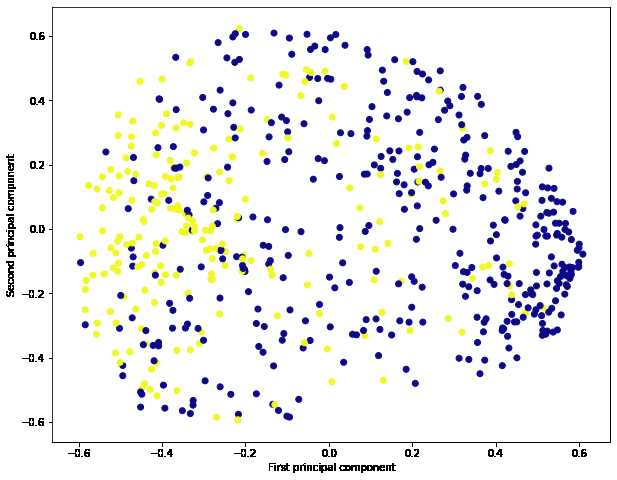
# 【2】SVC

from sklearn.svm import SVC
from sklearn.metrics import classification_report, confusion_matrix

classifier = SVC(kernel = 'rbf')
classifier.fit(X_train_pca, Y_train)
C:\Anaconda3\lib\site-packages\sklearn\svm\base.py:193: FutureWarning: The default value of gamma will change from 'auto' to 'scale' in version 0.22 to account better for unscaled features. Set gamma explicitly to 'auto' or 'scale' to avoid this warning.
"avoid this warning.", FutureWarning)
SVC(C=1.0, cache_size=200, class_weight=None, coef0=0.0,
decision_function_shape='ovr', degree=3, gamma='auto_deprecated',
kernel='rbf', max_iter=-1, probability=False, random_state=None,
shrinking=True, tol=0.001, verbose=False)# 使用SVC预测生存
y_pred = classifier.predict(X_test_pca)
cm = confusion_matrix(Y_test, y_pred)
# cm
print(classification_report(Y_test, y_pred)) precision recall f1-score support
0 0.74 0.86 0.80 100
1 0.63 0.44 0.52 54
accuracy 0.71 154
macro avg 0.69 0.65 0.66 154
weighted avg 0.70 0.71 0.70 154# 使用 网格搜索 来提高模型 就是穷举法 遍历各种参数的组合形式
from sklearn.model_selection import GridSearchCV
# C越大,即对误分类的惩罚增大,准确率越高,但泛化能力弱
# gamma:float参数,默认为auto核函数系数,只对'rbf'、 ‘poly' 、 ‘sigmoid'有效。
param_grid = {'C':[0.1, 1, 10, 100], 'gamma':[1, 0.1, 0.01, 0.001]}
grid = GridSearchCV(SVC(),param_grid,refit=True,verbose = 2)
grid.fit(X_train_pca, Y_train)
#显示穷举后 最优的参数
print('穷举后 最优的参数: ',grid.best_estimator_)
# 预测
grid_predictions = grid.predict(X_test_pca)
# 分类报告
print(classification_report(Y_test,grid_predictions))C:\Anaconda3\lib\site-packages\sklearn\model_selection\_split.py:1978: FutureWarning: The default value of cv will change from 3 to 5 in version 0.22. Specify it explicitly to silence this warning.
warnings.warn(CV_WARNING, FutureWarning)
[Parallel(n_jobs=1)]: Using backend SequentialBackend with 1 concurrent workers.
[Parallel(n_jobs=1)]: Done 1 out of 1 | elapsed: 0.0s remaining: 0.0s
Fitting 3 folds for each of 16 candidates, totalling 48 fits
[CV] C=0.1, gamma=1 ..................................................
[CV] ................................... C=0.1, gamma=1, total= 0.0s
[CV] C=0.1, gamma=1 ..................................................
[CV] ................................... C=0.1, gamma=1, total= 0.0s
[CV] C=0.1, gamma=1 ..................................................
[CV] ................................... C=0.1, gamma=1, total= 0.0s
[CV] C=0.1, gamma=0.1 ................................................
[CV] ................................. C=0.1, gamma=0.1, total= 0.0s
[CV] C=0.1, gamma=0.1 ................................................
[CV] ................................. C=0.1, gamma=0.1, total= 0.0s
[CV] C=0.1, gamma=0.1 ................................................
[CV] ................................. C=0.1, gamma=0.1, total= 0.0s
[CV] C=0.1, gamma=0.01 ...............................................
[CV] ................................ C=0.1, gamma=0.01, total= 0.0s
[CV] C=0.1, gamma=0.01 ...............................................
[CV] ................................ C=0.1, gamma=0.01, total= 0.0s
[CV] C=0.1, gamma=0.01 ...............................................
[CV] ................................ C=0.1, gamma=0.01, total= 0.0s
[CV] C=0.1, gamma=0.001 ..............................................
[CV] ............................... C=0.1, gamma=0.001, total= 0.0s
[CV] C=0.1, gamma=0.001 ..............................................
[CV] ............................... C=0.1, gamma=0.001, total= 0.0s
[CV] C=0.1, gamma=0.001 ..............................................
[CV] ............................... C=0.1, gamma=0.001, total= 0.0s
[CV] C=1, gamma=1 ....................................................
[CV] ..................................... C=1, gamma=1, total= 0.0s
[CV] C=1, gamma=1 ....................................................
[CV] ..................................... C=1, gamma=1, total= 0.0s
[CV] C=1, gamma=1 ....................................................
[CV] ..................................... C=1, gamma=1, total= 0.0s
[CV] C=1, gamma=0.1 ..................................................
[CV] ................................... C=1, gamma=0.1, total= 0.0s
[CV] C=1, gamma=0.1 ..................................................
[CV] ................................... C=1, gamma=0.1, total= 0.0s
[CV] C=1, gamma=0.1 ..................................................
[CV] ................................... C=1, gamma=0.1, total= 0.0s
[CV] C=1, gamma=0.01 .................................................
[CV] .................................. C=1, gamma=0.01, total= 0.0s
[CV] C=1, gamma=0.01 .................................................
[CV] .................................. C=1, gamma=0.01, total= 0.0s
[CV] C=1, gamma=0.01 .................................................
[CV] .................................. C=1, gamma=0.01, total= 0.0s
[CV] C=1, gamma=0.001 ................................................
[CV] ................................. C=1, gamma=0.001, total= 0.0s
[CV] C=1, gamma=0.001 ................................................
[CV] ................................. C=1, gamma=0.001, total= 0.0s
[CV] C=1, gamma=0.001 ................................................
[CV] ................................. C=1, gamma=0.001, total= 0.0s
[CV] C=10, gamma=1 ...................................................
[CV] .................................... C=10, gamma=1, total= 0.0s
[CV] C=10, gamma=1 ...................................................
[CV] .................................... C=10, gamma=1, total= 0.0s
[CV] C=10, gamma=1 ...................................................
[CV] .................................... C=10, gamma=1, total= 0.0s
[CV] C=10, gamma=0.1 .................................................
[CV] .................................. C=10, gamma=0.1, total= 0.0s
[CV] C=10, gamma=0.1 .................................................
[CV] .................................. C=10, gamma=0.1, total= 0.0s
[CV] C=10, gamma=0.1 .................................................
[CV] .................................. C=10, gamma=0.1, total= 0.0s
[CV] C=10, gamma=0.01 ................................................
[CV] ................................. C=10, gamma=0.01, total= 0.0s
[CV] C=10, gamma=0.01 ................................................
[CV] ................................. C=10, gamma=0.01, total= 0.0s
[CV] C=10, gamma=0.01 ................................................
[CV] ................................. C=10, gamma=0.01, total= 0.0s
[CV] C=10, gamma=0.001 ...............................................
[CV] ................................ C=10, gamma=0.001, total= 0.0s
[CV] C=10, gamma=0.001 ...............................................
[CV] ................................ C=10, gamma=0.001, total= 0.0s
[CV] C=10, gamma=0.001 ...............................................
[CV] ................................ C=10, gamma=0.001, total= 0.0s
[CV] C=100, gamma=1 ..................................................
[CV] ................................... C=100, gamma=1, total= 0.0s
[CV] C=100, gamma=1 ..................................................
[CV] ................................... C=100, gamma=1, total= 0.0s
[CV] C=100, gamma=1 ..................................................
[CV] ................................... C=100, gamma=1, total= 0.0s
[CV] C=100, gamma=0.1 ................................................
[CV] ................................. C=100, gamma=0.1, total= 0.0s
[CV] C=100, gamma=0.1 ................................................
[CV] ................................. C=100, gamma=0.1, total= 0.0s
[CV] C=100, gamma=0.1 ................................................
[CV] ................................. C=100, gamma=0.1, total= 0.0s
[CV] C=100, gamma=0.01 ...............................................
[CV] ................................ C=100, gamma=0.01, total= 0.0s
[CV] C=100, gamma=0.01 ...............................................
[CV] ................................ C=100, gamma=0.01, total= 0.0s
[CV] C=100, gamma=0.01 ...............................................
[CV] ................................ C=100, gamma=0.01, total= 0.0s
[CV] C=100, gamma=0.001 ..............................................
[CV] ............................... C=100, gamma=0.001, total= 0.0s
[CV] C=100, gamma=0.001 ..............................................
[CV] ............................... C=100, gamma=0.001, total= 0.0s
[CV] C=100, gamma=0.001 ..............................................
[CV] ............................... C=100, gamma=0.001, total= 0.0s
穷举后 最优的参数: SVC(C=10, cache_size=200, class_weight=None, coef0=0.0,
decision_function_shape='ovr', degree=3, gamma=1, kernel='rbf', max_iter=-1,
probability=False, random_state=None, shrinking=True, tol=0.001,
verbose=False)
precision recall f1-score support
0 0.73 0.89 0.80 100
1 0.66 0.39 0.49 54
accuracy 0.71 154
macro avg 0.69 0.64 0.65 154
weighted avg 0.70 0.71 0.69 154
[Parallel(n_jobs=1)]: Done 48 out of 48 | elapsed: 0.2s finishedax = sns.boxplot(data = results)
ax.set_xticklabels(names)[Text(0, 0, 'LR'),
Text(0, 0, 'NB'),
Text(0, 0, 'KNN'),
Text(0, 0, 'DT'),
Text(0, 0, 'SVM')]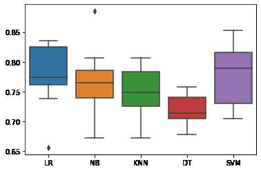
# 使用逻辑回归预测

lr = LogisticRegression() # LR模型构建
lr.fit(X_train, Y_train) #
predictions = lr.predict(X_test) # 使用测试值预测
C:\Anaconda3\lib\site-packages\sklearn\linear_model\logistic.py:432: FutureWarning: Default solver will be changed to 'lbfgs' in 0.22. Specify a solver to silence this warning.
FutureWarning)print(accuracy_score(Y_test, predictions)) # 打印评估指标(分类准确率)0.7142857142857143print(classification_report(Y_test,predictions)) precision recall f1-score support
0 0.73 0.88 0.80 100
1 0.65 0.41 0.50 54
accuracy 0.71 154
macro avg 0.69 0.64 0.65 154
weighted avg 0.70 0.71 0.69 154conf = confusion_matrix(Y_test, predictions) # 混淆矩阵label = ["0","1"] #
sns.heatmap(conf, annot = True, xticklabels=label, yticklabels=label)<matplotlib.axes._subplots.AxesSubplot at 0x1f2bbd44a48>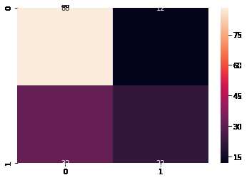
数据分析训练-Pima印第安人数据集上的机器学习-分类算法(根据诊断措施预测糖尿病的发病)
标签:obj arc body anova 控制 位置 功能 穷举 通过
原文地址:https://www.cnblogs.com/duoba/p/12392883.html