标签:tag ext fine class role lse 调整 情况下 m60
当模型层数增加到某种程度,模型的效果将会不升反降,发生退化。
不是过拟合:训练误差也大
不是梯度消失/爆炸:BN基本解决了这个问题
问题:堆加新的层后,这些层很难做到恒等映射,由于非线性激活。
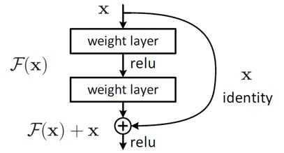
把网络设计为H(x) = F(x) + x,即直接把恒等映射作为网络的一部分。就可以把问题转化为学习一个残差函数F(x) = H(x) - x. 只要F(x)=0,就构成了一个恒等映射H(x) = x。 而且,拟合残差至少比拟合恒等映射容易得多。
用数学语言描述,假设Residual Block的输入为 ,则输出
等于:
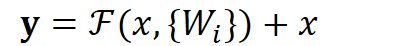
其中 是我们学习的目标,即输出输入的残差
。以上图为例,残差部分是中间有一个Relu激活的双层权重,即:
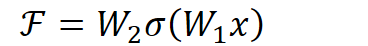
其中 指代Relu,而
指代两层权重。
顺带一提,这里一个Block中必须至少含有两个层,否则就会出现很滑稽的情况:

显然这样加了和没加差不多……
结构参考

ResNet是仿照VGG-19,只不过改变具体最小单元。
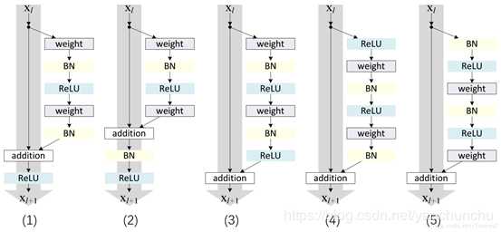
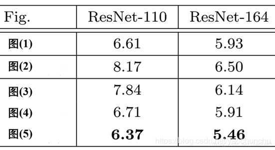
1 是原文中采用, 5 是改进版
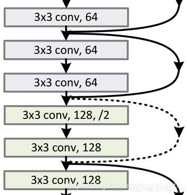
维度不一致体现在两个层面:
空间上不一致很简单,只需要在跳接的部分给输入x加上一个线性映射 ,即:

而对于深度上的不一致,则有两种解决办法,一种是在跳接过程中加一个1*1的卷积层进行升维,另一种则是直接简单粗暴地补零。事实证明两种方法都行得通。
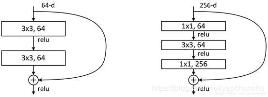
这两种结构分别针对ResNet34(左图)和ResNet50/101/152(右图),一般称整个结构为一个”building block“。其中右图又称为”bottleneck design”,目的一目了然,就是为了降低参数的数目。看右图,输入是一个3×3×256的特征,第一个步骤用64个1x1的卷积把256维channel降到64维,然后在最后通过1x1卷积恢复到256个channel,整体上用的参数数目:1x1x256x64 + 3x3x64x64 + 1x1x64x256 = 69632,而不使用bottleneck的话参考左图,输入假设是3x3x256,第一步经过256个卷积核3×3×256,第二部再经过256个卷积核3×3×256。所以参数数目: 3x3x256x256x2 = 1179648,差了16.94倍。
总体结构
def inference(hypes, images, train=True,
              num_classes=1000,
              num_blocks=[3, 4, 6, 3],  # defaults to 50-layer network
  preprocess=True,
              bottleneck=True):
    # if preprocess is True, input should be RGB [0,1], otherwise BGR with mean
 # subtracted
  layers = hypes[‘arch‘][‘layers‘]

    if layers == 50:
        num_blocks = [3, 4, 6, 3]
    elif layers == 101:
        num_blocks = [3, 4, 23, 3]
    elif layers == 152:
        num_blocks = [3, 8, 36, 3]
    else:
        assert()

    # 减均值,调顺序
  if preprocess:
        x = _imagenet_preprocess(images)

    is_training = tf.convert_to_tensor(train,
                                       dtype=‘bool‘,
                                       name=‘is_training‘)

    logits = {}

    with tf.variable_scope(‘scale1‘):
        x = _conv(x, 64, ksize=7, stride=2)
        x = _bn(x, is_training, hypes)
        x = _relu(x)
        scale1 = x

    with tf.variable_scope(‘scale2‘):
        x = _max_pool(x, ksize=3, stride=2)
        x = stack(x, num_blocks[0], 64, bottleneck, is_training, stride=1,
                  hypes=hypes)
        scale2 = x

    with tf.variable_scope(‘scale3‘):
        x = stack(x, num_blocks[1], 128, bottleneck, is_training, stride=2,
                  hypes=hypes)
        scale3 = x

    with tf.variable_scope(‘scale4‘):
        x = stack(x, num_blocks[2], 256, bottleneck, is_training, stride=2,
                  hypes=hypes)
        scale4 = x

    with tf.variable_scope(‘scale5‘):
        x = stack(x, num_blocks[3], 512, bottleneck, is_training, stride=2,
                  hypes=hypes)
        scale5 = x

    logits[‘deep_feat‘] = scale5

    logits[‘early_feat‘] = scale3

    if train:
        restore = tf.global_variables()
        hypes[‘init_function‘] = _initalize_variables
        hypes[‘restore‘] = restore

    return logits
每一个尺度scale下
def stack(x, num_blocks, filters_internal, bottleneck, is_training, stride,
          hypes):
    for n in range(num_blocks):
        s = stride if n == 0 else 1
  with tf.variable_scope(‘block%d‘ % (n + 1)):
            x = block(x,
                      filters_internal,
                      bottleneck=bottleneck,
                      is_training=is_training,
                      stride=s,
                      hypes=hypes)
    return x
具体到每个残差单元
def block(x, filters_internal, is_training, stride, bottleneck, hypes):
    filters_in = x.get_shape()[-1]
    # Note: filters_out isn‘t how many filters are outputed.
    # That is the case when bottleneck=False but when bottleneck is
    # True, filters_internal*4 filters are outputted. filters_internal
    # is how many filters
    # the 3x3 convs output internally.
    if bottleneck:
        filters_out = 4 * filters_internal
    else:
        filters_out = filters_internal

    shortcut = x  # branch 1

    if bottleneck:
        with tf.variable_scope(‘a‘):
            x = _conv(x, filters_internal, ksize=1, stride=stride)
            x = _bn(x, is_training, hypes)
            x = _relu(x)

        with tf.variable_scope(‘b‘):
            x = _conv(x, filters_internal, ksize=3, stride=1)
            x = _bn(x, is_training, hypes)
            x = _relu(x)

        with tf.variable_scope(‘c‘):
            x = _conv(x, filters_out, ksize=1, stride=1)
            x = _bn(x, is_training, hypes)
    else:
        with tf.variable_scope(‘A‘):
            x = _conv(x, filters_internal, ksize=3, stride=stride)
            x = _bn(x, is_training, hypes)
            x = _relu(x)

        with tf.variable_scope(‘B‘):
            x = _conv(x, filters_out, ksize=3, stride=1)
            x = _bn(x, is_training, hypes)

    with tf.variable_scope(‘shortcut‘):
        if filters_out != filters_in or stride != 1:
            shortcut = _conv(shortcut, filters_out, ksize=1, stride=stride)
            shortcut = _bn(shortcut, is_training, hypes)

    return _relu(x + shortcut)
R G B 每通道减去均值 (R_mean,G_mean,B_mean,均值为总样本统计得到的。
从主成分分析(PCA)入手解释
可以移除图像的平均亮度值。很多情况下我们对图像的照度并不感兴趣,而更多地关注其内容,比如在对象识别任务中,图像的整体明亮程度并不会影响图像中存在的是什么物体。
从反向传播计算入手
如果输入层 很大,在反向传播时候传递到输入层的梯度就会变得很大。
值得一提自然界图像平均RGB为120左右。理论上RGB是统计训练集的,本着测试集与其分开规则。然而由于Imagenet图片海量,可以直接用其统计的RGB。
IMAGENET_MEAN_BGR = [103.062623801, 115.902882574, 123.151630838, ]
def _imagenet_preprocess(rgb):
    """Changes RGB [0,1] valued image to BGR [0,255] with mean subtracted."""
    red, green, blue = tf.split(
        axis=3, num_or_size_splits=3, value=rgb * 255.0)
    bgr = tf.concat(axis=3, values=[blue, green, red])
    bgr -= IMAGENET_MEAN_BGR
return bgrBatch Normalization原理与实战
深度学习中 Batch Normalization为什么效果好?
一方面,当底层网络中参数发生微弱变化时,由于每一层中的线性变换与非线性激活映射,这些微弱变化随着网络层数的加深而被放大(类似蝴蝶效应);另一方面,参数的变化导致每一层的输入分布会发生改变,进而上层的网络需要不停地去适应这些分布变化,使得我们的模型训练变得困难。上述这一现象叫做Internal Covariate Shift。
当使用PCA白化时,可以使输入特征分布具有相同的均值与方差(均值为0,方差为1)
但计算成本高,且改变了每一层分布,丢失原始表达能力
BN的改进:
1、单独对每个特征进行normalizaiton就可以了,让每个特征都有均值为0,方差为1的分布。
2、再加个线性变换操作,让这些数据再能够尽可能恢复本身的表达能力。
标签:tag ext fine class role lse 调整 情况下 m60
原文地址:https://www.cnblogs.com/Caiyi-Xu/p/12513250.html