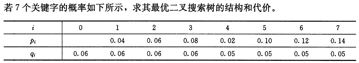
标签:euc precision 限制 may 变量 形式 领域 多少 cbe
# Colab 相关设置项
# Mount Google Drive
from google.colab import drive # import drive from google colab

ROOT = "/content/drive"     # default location for the drive
drive.mount(ROOT)           # we mount the google drive at /content/drive
# change to clrs directionary
%cd "/content/drive/My Drive/Colab Notebooks/CLRS/CLRS_notes"
Drive already mounted at /content/drive; to attempt to forcibly remount, call drive.mount("/content/drive", force_remount=True).
/content/drive/My Drive/Colab Notebooks/CLRS/CLRS_notes
%mkdir ch15
mkdir: cannot create directory ‘ch15’: File exists
import imp
import random
%%writefile ch15/cut_rod.py
"""钢条切割问题"""

def cut_rod(p, n):
  if n == 0:
    return 0
  q = float(‘-inf‘)
  for i in range(1, n+1):
    q = max(q, p[i-1] + cut_rod(p, n-i))
  return q
Overwriting ch15/cut_rod.py
import ch15.cut_rod
from ch15.cut_rod import cut_rod
p = [1, 5, 8, 9, 10, 17, 17, 20, 24, 30]
cut_rod(p, 4)
10
%%writefile -a ch15/cut_rod.py


def memoized_cut_rod(p, n):
  """带备忘发的自顶向下法"""
  r = [float(‘-inf‘)] * (n+1)
  return memoized_cut_rod_aux(p, n, r)


def memoized_cut_rod_aux(p, n, r):
  """"带备忘录的自顶向下法的辅助函数"""
  if r[n] >=0:
    return r[n]
  if n == 0:
    q = 0
  else:
    q = float(‘-inf‘)
    for i in range(1, n+1):
      q = max(q, p[i-1] + memoized_cut_rod_aux(p, n-i, r))
  r[n] = q
  return q
Appending to ch15/cut_rod.py
imp.reload(ch15.cut_rod)
from ch15.cut_rod import memoized_cut_rod
p = [1, 5, 8, 9, 10, 17, 17, 20, 24, 30]
memoized_cut_rod(p, 4)
10
%%writefile -a ch15/cut_rod.py


def bottom_up_cut_rod(p, n):
  """自底向上法"""
  r = [float(‘-inf‘)] * (n + 1)
  r[0] = 0
  for i in range(1, n+1):
    q = float(‘-inf‘)
    for j in range(1, i+1):
      q = max(q, p[j-1] + r[i-j])
    r[i] = q
  return r[-1]
Appending to ch15/cut_rod.py
imp.reload(ch15.cut_rod)
from ch15.cut_rod import bottom_up_cut_rod
p = [1, 5, 8, 9, 10, 17, 17, 20, 24, 30]
bottom_up_cut_rod(p, 4)
10
%%writefile -a ch15/cut_rod.py


def extend_bottom_up_cut_rod(p, n):
  """保存最优切割方案"""
  r = [float(‘-inf‘)] * (n+1)  # 存放最优收益
  s = [0] * n  # 保留最佳切割方案
  r[0] = 0
  for i in range(1, n+1):
    for j in range(1, i+1):
      if r[i] < p[j-1] + r[i-j]:
        r[i] = p[j-1] + r[i-j]
        s[i-1] = j
  return r, s


def print_cut_rod(s, n=None):
  """打印出最佳切割方案"""
  n = len(s) - 1 if n == None else n
  while n >= 0:
    print(s[n], end=" ")
    n = n - s[n]
Appending to ch15/cut_rod.py
import ch15.cut_rod
imp.reload(ch15.cut_rod)
from ch15.cut_rod import print_cut_rod, extend_bottom_up_cut_rod
p = [1, 5, 8, 9, 10, 17, 17, 20, 24, 30]
_, s = extend_bottom_up_cut_rod(p, 7)
print_cut_rod(s)
1 6

可采用数学归纳法证明
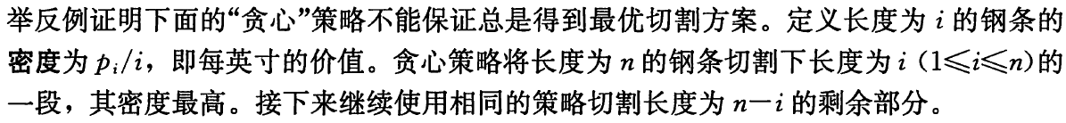
当 \(n=4\) 时,如果采用贪心法,方案为 3 + 1, 收益为 9。而最优方案为 2 + 2, 收益为 10

切割成本为 \(c\), 相当于需要添加选择成本
%%writefile -a ch15/cut_rod.py


def cut_rod_with_cost(p, n, c):
  """练习题 15.1-3,需要考虑切割成本"""
  r = [float(‘-inf‘)] * (n+1)
  s = [0] * n
  r[0] = c  # 避免后续判断是否需要加上切割成本
  for i in range(1, n+1):
    for j in range(1, i+1):
      t = p[j-1] + r[i-j] - c
      if t > r[i]:
        r[i] = t
        s[i-1] = j
  return r, s
Appending to ch15/cut_rod.py
import ch15.cut_rod
imp.reload(ch15.cut_rod)
from ch15.cut_rod import cut_rod_with_cost, print_cut_rod
p = [1, 5, 8, 9, 10, 17, 17, 20, 24, 30]
r, s = cut_rod_with_cost(p, 10, 1)
r[1:]
[1, 5, 8, 9, 12, 17, 17, 21, 24, 30]
s
[1, 2, 3, 2, 2, 6, 1, 2, 3, 10]

%%writefile -a ch15/cut_rod.py


def extend_memoized_cut_rod(p, n):
  """返回切割方案的带备忘发的自顶向下法"""
  r = [float(‘-inf‘)] * (n+1)
  s = [0] * n
  extend_memoized_cut_rod_aux(p, n, r, s)
  return r, s


def extend_memoized_cut_rod_aux(p, n, r, s):
  """"返回切割方案的带备忘录的自顶向下法的辅助函数"""
  if r[n] >=0:
    return r[n]
  if n == 0:
    q = 0
  else:
    q = float(‘-inf‘)
    for i in range(1, n+1):
      t = p[i-1] + extend_memoized_cut_rod_aux(p, n-i, r, s)
      if t > q:
        q = t
        s[n-1] = i
  r[n] = q
  return q
Appending to ch15/cut_rod.py
import ch15.cut_rod
imp.reload(ch15.cut_rod)
from ch15.cut_rod import extend_memoized_cut_rod, print_cut_rod
p = [1, 5, 8, 9, 10, 17, 17, 20, 24, 30]
r, s = extend_memoized_cut_rod(p, 7)
print("最优收益为: ", r[-1])
print("最优切割方案为")
print_cut_rod(s)
最优收益为:  18
最优切割方案为
1 6

使用一张表储存前 \(n-1\) 个计算的斐波那契数即可
%%writefile ch15/fibonacci.py
def fibonacci(n):
  """使用动态规划法计算斐波那契数列"""
  if n == 0: return 0
  if n == 1: return 1
  r = [0] * (n+1)
  r[0], r[1] = 0, 1
  for i in range(2, n+1):
    r[i] = r[i-1] + r[i-2]
  return r[-1]
Overwriting ch15/fibonacci.py
from ch15.fibonacci import fibonacci
for i in range(11):
  print(fibonacci(i), end=" ")
0 1 1 2 3 5 8 13 21 34 55
&\left(A_{1}\left(\left(A_{2} A_{3}\right) A_{4}\right)\right)\
&\left(\left(A_{1} A_{2}\right)\left(A_{3} A_{4}\right)\right)\
&\left(\left(A_{1}\left(A_{2} A_{3}\right)\right) A_{4}\right)\
&\left(\left(\left(A_{1} A_{2}\right) A_{3}\right) A_{4}\right)
\end{align}$$
矩阵乘法所需的乘法次数
矩阵链乘法问题
\sum_{k=1}^{n-1} P(k) P(n-k) & if\ n \ge 2
\end{array}\right.$$
动态规划的第一步是寻找最优子结构
对于矩阵链乘法问题,最优子结构如下:
利用最优子结构性质从子问题的最优解构造原问题的最优解
\min \limits_{i \leq k<j}\left{m[i, k]+m[k+1, j]+p_{i-1} p_{k} p_{j}\right} & \text { if } i<j
\end{array}\right.$$
%%writefile ch15/matrix_chain.py
""""矩阵链乘法的动态规划算法"""
def matrix_chain_order(p):
  """计算矩阵链乘法所需要的最少标量乘法"""
  length = len(p) - 1  # 矩阵链中矩阵的个数
  m = [[ 0 for i in range(length)] for j in range(length)]  # 存放 m[i, j] 的最优解
  s = [[ 0 for i in range(length-1)] for j in range(length-1)]  # 存放 m[i, j](i < j)最优解对应的分割点 k , 其中 m[i, j] 对应的值存放在 s[i, j-1] 中
  for matrix_length in range(2, length+1):
    for i in range(1, length - matrix_length + 2):
      j = i + matrix_length - 1
      m[i-1][j-1] = float(‘inf‘)
      for k in range(i, j):
        q = m[i-1][k-1] + m[k][j-1] + p[i-1]*p[k]*p[j]
        if q < m[i-1][j-1]:
          m[i-1][j-1] = q
          s[i-1][j-2] = k
  return m, s
Overwriting ch15/matrix_chain.py
import ch15.matrix_chain
from ch15.matrix_chain import matrix_chain_order
p = [30, 35, 15, 5, 10, 20, 25]
m, s = matrix_chain_order(p)
m
[[0, 15750, 7875, 9375, 11875, 15125],
 [0, 0, 2625, 4375, 7125, 10500],
 [0, 0, 0, 750, 2500, 5375],
 [0, 0, 0, 0, 1000, 3500],
 [0, 0, 0, 0, 0, 5000],
 [0, 0, 0, 0, 0, 0]]
s
[[1, 1, 3, 3, 3],
 [0, 2, 3, 3, 3],
 [0, 0, 3, 3, 3],
 [0, 0, 0, 4, 5],
 [0, 0, 0, 0, 5]]
%%writefile -a ch15/matrix_chain.py


def print_optimal_parents(s, i, j):
  """根据矩阵 s 中的信息,打印出最优化的括号方案"""
  if i == j:
    print("A{}".format(i), end="")
  else:
    print("(", end="")
    print_optimal_parents(s, i, s[i-1][j-2])
    print_optimal_parents(s, s[i-1][j-2]+1, j)
    print(")", end="")
Appending to ch15/matrix_chain.py
imp.reload(ch15.matrix_chain)
from ch15.matrix_chain import print_optimal_parents, matrix_chain_order
p = [30, 35, 15, 5, 10, 20, 25]
m, s = matrix_chain_order(p)
print_optimal_parents(s, 1, len(p)-1)
((A1(A2A3))((A4A5)A6))

import ch15.matrix_chain
imp.reload(ch15.matrix_chain)
from ch15.matrix_chain import print_optimal_parents, matrix_chain_order
p = [5, 10, 3, 12, 5, 50, 6]
m, s = matrix_chain_order(p)
print_optimal_parents(s, 1, len(p)-1)
((A1A2)((A3A4)(A5A6)))
m[0][-1]
2010
%%writefile -a ch15/matrix_chain.py


def matrix_chain_multiply(A, s, i, j):
  """计算矩阵链的乘积"""
  if i == j:
    return A[i-1]
  l = matrix_chain_multiply(A, s, i, s[i-1][j-2])
  r = matrix_chain_multiply(A, s, s[i-1][j-2]+1, j)
  return [[ sum([l[i][k] * r[k][j] for k in range(len(l[0]))])  # 计算两个矩阵的乘积
        for j in range(len(r[0]))]
        for i in range(len(l))]
Appending to ch15/matrix_chain.py
import ch15.matrix_chain
imp.reload(ch15.matrix_chain)
from ch15.matrix_chain import print_optimal_parents, matrix_chain_order, matrix_chain_multiply

from functools import reduce
import numpy as np  # 利用 numpy 判断计算结果是否正确
p = [5, 10, 3, 12, 5, 50, 6]
A = []
for index, item in enumerate(p[:-1], 1):
  A.append(np.random.randint(0, 10, (item, p[index])))
m, s = matrix_chain_order(p)
(matrix_chain_multiply(A, s, 1, len(A)) == reduce(np.dot, A)).all()
True

递推公式如下:
\sum_{k=1}^{n-1} P(k) P(n-k) & \text { if } n \geq 2
\end{array}\right.$$

子问题图的顶点个数为:
对于 \(A_{i..j}\) 的矩阵链,其需求解的子问题数为 \(2(j-i)\),所以包含的边数为:
&= \sum_{i=1}^{n-1}{i(i+1) = {n(n-1)(n+1) \over 3}} && 此处可通过归纳法证明
\end{align}$$
这些边连接一个问题所需要求解的子问题

此问题的解即为问题 15.2-4 中的子问题图中的边的总数目

可通过归纳法进行证明
对于 \(n=1\),不需要进行括号化,需要 $n-1 = 0 $ 对括号,符合要求
假设 \(\forall 0 \le x \lt n\),其完全括号化需要 \(x-1\) 对括号
则当有 \(n\) 个元素时,在第 \(k\) 个元素添加括号,可得到完全括号化方案。则 \(A_{1..k}\) 有 \(k-2\) 对括号, \(A_{k+1..n}\) 有 \(n-k-1\) 对括号,在 \(k\) 处分割会引入两对括号,由此可得需要的总括号对数为:

RECURSIVE-MATRIX-CHAIN 方法较优
对于 \(A_{1..n}\) 来说,假设 第 \(k\) 个元素是其最优的分割点

递归调用树如下
备忘技术对分治算法无效,主要是因为分治算法每步产生的子问题都是新的子问题,想互之间不重叠

任然具有最优子结构的性质,假设 \(k\) 为 \(A_{1..n}\) 的最优分割点
则 \(A_{1..k}\) 和 \(A{k+1..n}\) 也需要为最大化矩阵序列括号化方案,才能得到总体的最大化矩阵序列括号化方案

设 \(p = [1000,100,20,10,1000]\)
则按照题述的方法,最优的括号化方案为 \(\left(\left(\left(A_{1} A_{2}\right) A_{3}\right) A_{4}\right)\)
完全括号化方案为 \(\left(\left(A_{1}\left(A_{2} A_{3}\right)\right) A_{4}\right)\)

证明:
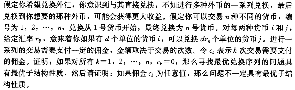
佣金为 \(0\)
佣金 \(c_k\) 可能为任意值
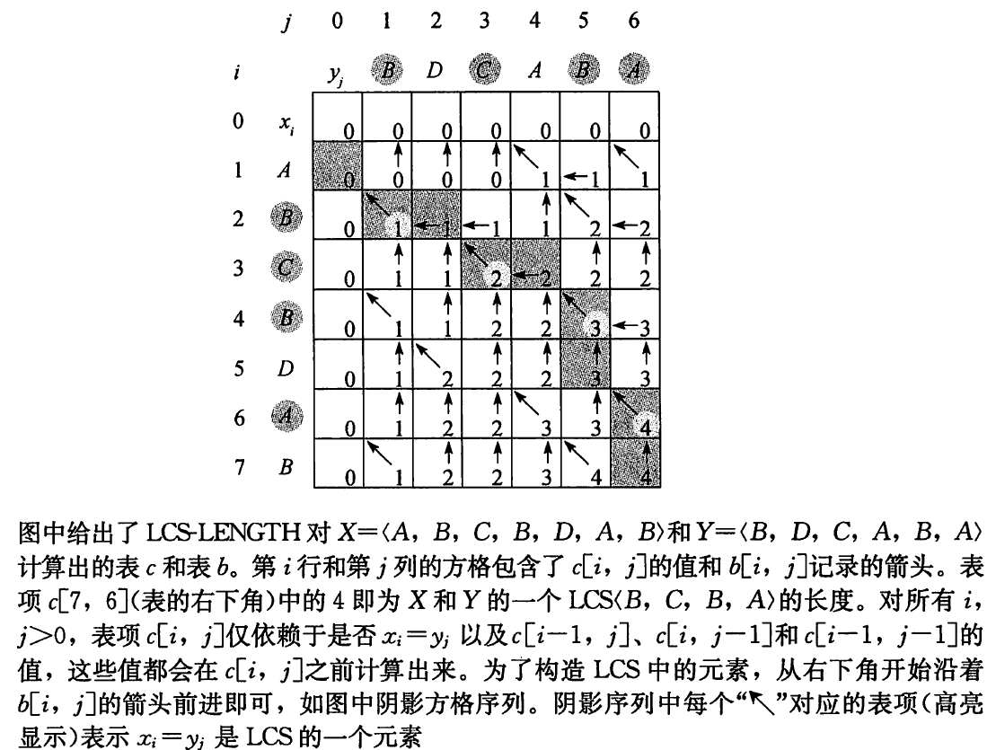
%%writefile ch15/lcs.py
"""最长公共子序列问题"""


def lcs_length(X, Y):
  """求两个序列的最长公共子序列"""
  m, n = len(X), len(Y)
  c = [[0]*(n+1) for i in range(m+1)]
  b = [[None]*n for i in range(m)]
  for i in range(1, m+1):
    for j in range(1, n+1):
      if X[i-1] == Y[j-1]:
        c[i][j] = c[i-1][j-1] + 1
        b[i-1][j-1] = ‘↖‘
      elif c[i-1][j] >= c[i][j-1]:
        c[i][j] = c[i-1][j]
        b[i-1][j-1] = ‘↑‘
      else:
        c[i][j] = c[i][j-1]
        b[i-1][j-1] = ‘←‘
  return c, b
Overwriting ch15/lcs.py
import ch15.lcs
imp.reload(ch15.lcs)
from ch15.lcs import lcs_length
X = [‘A‘, ‘B‘, ‘C‘, ‘B‘, ‘D‘, ‘A‘, ‘B‘]
Y = [‘B‘, ‘D‘, ‘C‘, ‘A‘, ‘B‘, ‘A‘]
c, b = lcs_length(X, Y)
c
[[0, 0, 0, 0, 0, 0, 0],
 [0, 0, 0, 0, 1, 1, 1],
 [0, 1, 1, 1, 1, 2, 2],
 [0, 1, 1, 2, 2, 2, 2],
 [0, 1, 1, 2, 2, 3, 3],
 [0, 1, 2, 2, 2, 3, 3],
 [0, 1, 2, 2, 3, 3, 4],
 [0, 1, 2, 2, 3, 4, 4]]
b
[[‘↑‘, ‘↑‘, ‘↑‘, ‘↖‘, ‘←‘, ‘↖‘],
 [‘↖‘, ‘←‘, ‘←‘, ‘↑‘, ‘↖‘, ‘←‘],
 [‘↑‘, ‘↑‘, ‘↖‘, ‘←‘, ‘↑‘, ‘↑‘],
 [‘↖‘, ‘↑‘, ‘↑‘, ‘↑‘, ‘↖‘, ‘←‘],
 [‘↑‘, ‘↖‘, ‘↑‘, ‘↑‘, ‘↑‘, ‘↑‘],
 [‘↑‘, ‘↑‘, ‘↑‘, ‘↖‘, ‘↑‘, ‘↖‘],
 [‘↖‘, ‘↑‘, ‘↑‘, ‘↑‘, ‘↖‘, ‘↑‘]]
%%writefile -a ch15/lcs.py


def print_LCS(b, X, i, j):
  """打印出最长公共子序列"""
  if i == 0 or j == 0:
    return
  if b[i-1][j-1] == ‘↖‘:
    print_LCS(b, X, i-1, j-1)
    print(X[i-1], end=" ")
  elif b[i-1][j-1] == ‘↑‘:
    print_LCS(b, X, i-1, j)
  else:
    print_LCS(b, X, i, j-1)
Appending to ch15/lcs.py
import ch15.lcs
imp.reload(ch15.lcs)
from ch15.lcs import lcs_length, print_LCS
X = [‘A‘, ‘B‘, ‘C‘, ‘B‘, ‘D‘, ‘A‘, ‘B‘]
Y = [‘B‘, ‘D‘, ‘C‘, ‘A‘, ‘B‘, ‘A‘]
c, b = lcs_length(X, Y)
print_LCS(b, X, len(X), len(Y))
B C B A

import ch15.lcs
imp.reload(ch15.lcs)
from ch15.lcs import lcs_length, print_LCS
X = [1, 0, 0, 1, 0, 1, 0, 1]
Y = [0, 1, 0, 1, 1, 0, 1, 1, 0]
c, b = lcs_length(X, Y)
print_LCS(b, X, len(X), len(Y))
1 0 0 1 1 0

%%writefile -a ch15/lcs.py


def print_LCS_without_b(c, X, Y, i, j):
  """15.4-2: 在没有表 b 的情况下输出最长公共子序列"""
  if i == 0 or j == 0:
    return
  if c[i][j] == c[i-1][j-1] + 1:
    print_LCS_without_b(c, X, Y, i-1, j-1)
    print(X[i-1], end=‘ ‘)
  elif c[i][j] == c[i-1][j]:
    print_LCS_without_b(c, X, Y, i-1, j)
  else:
    print_LCS_without_b(c, X, Y, i, j-1)
Appending to ch15/lcs.py
import ch15.lcs
imp.reload(ch15.lcs)
from ch15.lcs import lcs_length, print_LCS_without_b
X = [1, 0, 0, 1, 0, 1, 0, 1]
Y = [0, 1, 0, 1, 1, 0, 1, 1, 0]
c, b = lcs_length(X, Y)
print_LCS_without_b(c, X, Y, len(X), len(Y))
1 0 1 0 1 1

%%writefile -a ch15/lcs.py


def memoized_lcs_length(X, Y):
  """15.4-3: 带备忘的 lcs 算法"""
  m, n = len(X), len(Y)
  c = [[None] * (n+1) for i in range(m+1)]
  b = [[None]* n for i in range(m)]
  memoized_lcs_length_aux(X, Y, len(X), len(Y), c, b)
  return c, b


def memoized_lcs_length_aux(X, Y, i, j, c, b):
  """带备忘的 lcs 算法的辅助函数"""
  if i == 0 or j == 0:
    return 0
  if X[i-1] == Y[j-1]:
    c[i][j] = 1 + memoized_lcs_length_aux(X, Y, i-1, j-1, c, b)
    b[i-1][j-1] = ‘↖‘
  else:
    up = memoized_lcs_length_aux(X, Y, i-1, j, c, b)
    left = memoized_lcs_length_aux(X, Y, i, j-1, c, b)
    b[i-1][j-1], c[i][j] = (‘↑‘, up) if up >= left else (‘←‘, left)
  return c[i][j]
Appending to ch15/lcs.py
import ch15.lcs
imp.reload(ch15.lcs)
from ch15.lcs import memoized_lcs_length, print_LCS
X = [‘A‘, ‘B‘, ‘C‘, ‘B‘, ‘D‘, ‘A‘, ‘B‘]
Y = [‘B‘, ‘D‘, ‘C‘, ‘A‘, ‘B‘, ‘A‘]
c, b = memoized_lcs_length(X, Y)
print_LCS(b, X, len(X), len(Y))
B C B A
b
[[‘↑‘, ‘↑‘, ‘↑‘, ‘↖‘, None, None],
 [‘↖‘, ‘←‘, ‘←‘, ‘↑‘, None, None],
 [‘↑‘, ‘↑‘, ‘↖‘, ‘←‘, None, None],
 [‘↖‘, ‘↑‘, ‘↑‘, ‘↑‘, ‘↖‘, None],
 [None, ‘↖‘, ‘↑‘, ‘↑‘, ‘↑‘, None],
 [None, None, None, ‘↖‘, None, ‘↖‘],
 [None, None, None, None, ‘↖‘, ‘↑‘]]
c
[[None, None, None, None, None, None, None],
 [None, 0, 0, 0, 1, None, None],
 [None, 1, 1, 1, 1, None, None],
 [None, 1, 1, 2, 2, None, None],
 [None, 1, 1, 2, 2, 3, None],
 [None, None, 2, 2, 2, 3, None],
 [None, None, None, None, 3, None, 4],
 [None, None, None, None, None, 4, 4]]

每次计算 \(c[i, j]\) 时,只需要利用 \(c[i-1, j-1], c[i-1, j], c[i, j-1]\) 这三个值即可,因此可以只储存之前一行和当前计算行的信息,便可完成计算
%%writefile -a ch15/lcs.py


from collections import deque


def lcs_length_queue(X, Y):
  """15.4-4: 借助队列来减小表项所需的额外空间"""
  m, n = len(X), len(Y)
  if m < n:
    m, n = n, m
    X, Y = Y, X
  dq = deque(maxlen=n)
  a = 0  # 初始时的 c[i-1][j-1]
  for i in range(m):
    for j in range(n):
      if X[i] == Y[j]:
        b = a + 1  if j != 0 else 1 # b 为 c[i][j]
        a = dq.popleft() if i != 0 else 0 # 下一次循环时的 c[i-1][j-1]
        dq.append(b)
      else:
        a = dq.popleft() if i != 0 else 0 # 此次循环的 c[i-1][j], 下一次循环的 c[i-1][j-1]
        d = dq[-1] if j != 0 else 0 # c[i][j-1]
        dq.append(max(a, d))
  return dq[-1]
Appending to ch15/lcs.py
import ch15.lcs
imp.reload(ch15.lcs)
from ch15.lcs import lcs_length_queue
X = [‘A‘, ‘B‘, ‘C‘, ‘B‘, ‘D‘, ‘A‘, ‘B‘]
Y = [‘B‘, ‘D‘, ‘C‘, ‘A‘, ‘B‘, ‘A‘]
lcs_length_queue(X, Y)
4
X = [1, 0, 0, 1, 0, 1, 0, 1]
Y = [0, 1, 0, 1, 1, 0, 1, 1, 0]
lcs_length_queue(X, Y)
6

设序列为 \(X\),将 \(X\) 中的元素按递增的顺序排列得到序列 \(Y\), 则 \(X\) 与 \(Y\) 的最大公共子序列即为 \(X\) 中最长的单调递增子序列
%%writefile -a ch15/lcs.py


def longest_increasing_subsequence_by_LCS(X):
  """15.4-5: 在 O(n^2) 的时间内求一个序列的最长单调递增子序列"""
  Y = sorted(X)
  c, b = memoized_lcs_length(X, Y)
  print_LCS(b, X, len(X), len(Y))
Appending to ch15/lcs.py
import ch15.lcs
imp.reload(ch15.lcs)
from ch15.lcs import longest_increasing_subsequence_by_LCS
X = list(range(10))
random.shuffle(X)
print(X, "中的最长单调递增子序列为: ")
longest_increasing_subsequence_by_LCS(X)
[8, 5, 7, 4, 1, 2, 6, 9, 3, 0] 中的最长单调递增子序列为:
1 2 6 9

提示描述的有问题,应为:
算法描述
%%writefile ch15/longest_increasing_subsequence.py


from bisect import bisect

def longest_increasing_subsequence(X):
  """15.4-6: 在 O(nlgn) 的时间内求解一个序列的最长单调递增子序列"""
  s = [float(‘inf‘)] * len(X)
  L = 0  # s 中非 inf 的元素数目
  for i in range(len(X)):
    j = bisect(s, X[i])
    s[j] = X[i]
    if j + 1 > L:
      L = j + 1
  res = [None] * L
  k = len(X)
  s.append(float(‘inf‘))
  for i in reversed(range(L)):
    while k > 0:
      k -= 1
      if s[i+1] >= X[k] >= s[i]:
        res[i] = X[k]
        break
  return res
Overwriting ch15/longest_increasing_subsequence.py
import ch15.longest_increasing_subsequence
imp.reload(ch15.longest_increasing_subsequence)
from ch15.longest_increasing_subsequence import longest_increasing_subsequence
X = list(range(10))
random.shuffle(X)
# X = [1, 2, 3, 4, 1, 2, 5, 4]
print(X, "中的最长单调递增子序列为: ", longest_increasing_subsequence(X))
[0, 4, 7, 2, 3, 5, 9, 8, 6, 1] 中的最长单调递增子序列为: [0, 2, 3, 5, 6]
&=1+\sum_{i=1}^{n} \operatorname{depth}{T}\left(k{i}\right) \cdot p_{i}+\sum_{i=0}^{n} \operatorname{depth}{T}\left(d{i}\right) \cdot q_{i}
\end{align}$$
\min _{i \leq r \leq j}{e[i, r-1]+e[r+1, j]+w(i, j)} & \text { if } i \leq j
\end{array}\right.$$
%%writefile ch15/optimal_bst.py
""""计算最优二叉搜索树"""


def optimal_bst(p, q):
  n = len(p)
  e = [[ q[i-1] if (i-1) == j else float(‘inf‘) for i in range(1, n+2)] for j in range(n+1)]
  w = [[ q[i-1] if (i-1) == j else 0 for i in range(1, n+2)] for j in range(n+1)]
  root = [[0] * n for i in range(n)]
  for l in range(1, n+1):
    for i in range(1, n-l+2):
      j = i + l - 1
      w[i-1][j] = w[i-1][j-1] + p[j-1] + q[j]
      for k in range(i, j+1):
        t = e[i-1][k-1] + e[k][j] + w[i-1][j]
        if t < e[i-1][j]:
          e[i-1][j] = t
          root[i-1][j-1] = k
  return e, root
Overwriting ch15/optimal_bst.py
import ch15.optimal_bst
imp.reload(ch15.optimal_bst)
from ch15.optimal_bst import optimal_bst
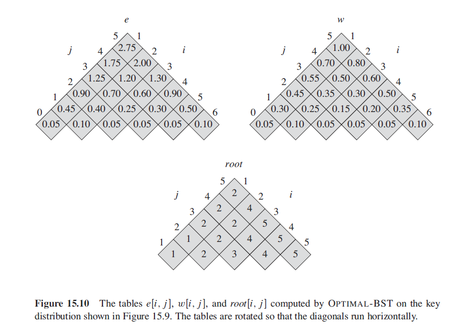
p = [0.15, 0.10, 0.05, 0.10, 0.20]
q = [0.05, 0.10, 0.05, 0.05, 0.05, 0.10]
e, root = optimal_bst(p, q)
e
[[0.05, 0.45000000000000007, 0.9, 1.25, 1.75, 2.75],
 [inf, 0.1, 0.4, 0.7, 1.2, 2.0],
 [inf, inf, 0.05, 0.25, 0.6, 1.2999999999999998],
 [inf, inf, inf, 0.05, 0.30000000000000004, 0.9],
 [inf, inf, inf, inf, 0.05, 0.5],
 [inf, inf, inf, inf, inf, 0.1]]
root
[[1, 1, 2, 2, 2],
 [0, 2, 2, 2, 4],
 [0, 0, 3, 4, 5],
 [0, 0, 0, 4, 5],
 [0, 0, 0, 0, 5]]
相当于中序遍历
%%writefile -a ch15/optimal_bst.py


def construct_optimal_bst(root):
  """15.5-1: 构造最优二叉搜索树"""
  m, n = len(root), len(root[0])
  print("k{} 为根".format(root[0][n-1]))
  construct_optimal_bst_aux(root, 1, n)


def construct_optimal_bst_aux(root, i, j):
  """构造最优二叉搜索树的辅助函数"""
  r = root[i-1][j-1]
  if i == j:
    print("d{} 为 k{} 的左孩子".format(r-1, r))
    print("d{} 为 k{} 的右孩子".format(r, r))
    return
  if i == r:
    print("d{} 为 k{} 的左孩子".format(r-1, r-1))
  else:
    print("k{} 为 k{} 的左孩子".format(root[i-1][r-2], r))
    construct_optimal_bst_aux(root, i, r-1)
  if j == r:
    print("d{} 为 d{} 的右孩子".format(r, r))
  else:
    print("k{} 为 k{} 的右孩子".format(root[r][j-1], r))
    construct_optimal_bst_aux(root, r+1, j)
Appending to ch15/optimal_bst.py
import ch15.optimal_bst
imp.reload(ch15.optimal_bst)
from ch15.optimal_bst import optimal_bst, construct_optimal_bst
p = [0.15, 0.10, 0.05, 0.10, 0.20]
q = [0.05, 0.10, 0.05, 0.05, 0.05, 0.10]
e, root = optimal_bst(p, q)
construct_optimal_bst(root)
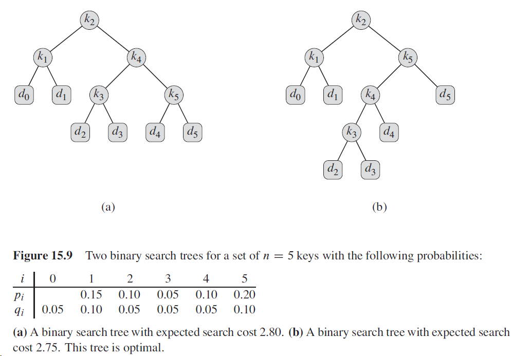
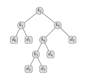
k2 为根
k1 为 k2 的左孩子
d0 为 k1 的左孩子
d1 为 k1 的右孩子
k5 为 k2 的右孩子
k4 为 k5 的左孩子
k3 为 k4 的左孩子
d2 为 k3 的左孩子
d3 为 k3 的右孩子
d4 为 d4 的右孩子
d5 为 d5 的右孩子
import ch15.optimal_bst
imp.reload(ch15.optimal_bst)
from ch15.optimal_bst import optimal_bst, construct_optimal_bst
p = [0.04, 0.06, 0.08, 0.02, 0.10, 0.12, 0.14]
q = [0.06, 0.06, 0.06, 0.06, 0.05, 0.05, 0.05, 0.05]
e, root = optimal_bst(p, q)
print("期望代价为:", e[0][-1])
期望代价为: 3.12
construct_optimal_bst(root)
k5 为根
k2 为 k5 的左孩子
k1 为 k2 的左孩子
d0 为 k1 的左孩子
d1 为 k1 的右孩子
k3 为 k2 的右孩子
d2 为 k2 的左孩子
k4 为 k3 的右孩子
d3 为 k4 的左孩子
d4 为 k4 的右孩子
k7 为 k5 的右孩子
k6 为 k7 的左孩子
d5 为 k6 的左孩子
d6 为 k6 的右孩子
d7 为 d7 的右孩子

公式 (15.12) 如下:
每次计算的时间代价为 \(O(n)\),因此不会影响渐近时间复杂性
%%writefile -a ch15/optimal_bst.py


def improved_optimal_bst(p, q):
  """15.5-4: 改进最优二叉搜索树算法"""
  n = len(p)
  e = [[ q[i-1] if (i-1) == j else float(‘inf‘) for i in range(1, n+2)] for j in range(n+1)]
  w = [[ q[i-1] if (i-1) == j else 0 for i in range(1, n+2)] for j in range(n+1)]
  root = [[0] * n for i in range(n)]
  for l in range(1, n+1):
    for i in range(1, n-l+2):
      j = i + l - 1
      w[i-1][j] = w[i-1][j-1] + p[j-1] + q[j]
      if i != j:
        r = range(root[i-1][j-2], root[i][j-1])  # 利用相关的结论
      else:
        r = range(i, j+1)
      for k in range(i, j+1):
        t = e[i-1][k-1] + e[k][j] + w[i-1][j]
        if t < e[i-1][j]:
          e[i-1][j] = t
          root[i-1][j-1] = k

  return e, root
Appending to ch15/optimal_bst.py
import ch15.optimal_bst
imp.reload(ch15.optimal_bst)
from ch15.optimal_bst import improved_optimal_bst
p = [0.15, 0.10, 0.05, 0.10, 0.20]
q = [0.05, 0.10, 0.05, 0.05, 0.05, 0.10]
e, root = improved_optimal_bst(p, q)
e
[[0.05, 0.45000000000000007, 0.9, 1.25, 1.75, 2.75],
 [inf, 0.1, 0.4, 0.7, 1.2, 2.0],
 [inf, inf, 0.05, 0.25, 0.6, 1.2999999999999998],
 [inf, inf, inf, 0.05, 0.30000000000000004, 0.9],
 [inf, inf, inf, inf, 0.05, 0.5],
 [inf, inf, inf, inf, inf, 0.1]]
root
[[1, 1, 2, 2, 2],
 [0, 2, 2, 2, 4],
 [0, 0, 3, 4, 5],
 [0, 0, 0, 4, 5],
 [0, 0, 0, 0, 5]]

涉及到图论的相关知识,学完图后再回来补
import ch15.lcs
imp.reload(ch15.lcs)
from ch15.lcs import lcs_length, print_LCS
X = ‘character‘
Y = X[::-1]
c, b = lcs_length(X, Y)
print_LCS(b, X, len(X), len(Y))
c a r a c
%%writefile ch15/longest_palindrome_subsequence.py
"""15-2 最长回文子序列"""


def longest_palindrome_subsequence(X):
  """空间复杂度为 O(n^3)"""
  n = len(X)
  c = [[‘‘ if i!=j else X[i] for j in range(n)] for i in range(n)]
  for l in range(2, n+1):
    for i in range(1, n-l+2):
      j = i + l - 1
      if X[i-1] == X[j-1]:
        c[i-1][j-1] = X[i-1] + c[i][j-2] + X[j-1]
      else:
        c[i-1][j-1] = c[i][j-1] if len(c[i][j-1]) > len(c[i-1][j-2]) else c[i-1][j-2]
  return c[0][n-1]
Overwriting ch15/longest_palindrome_subsequence.py
import ch15.longest_palindrome_subsequence
imp.reload(ch15.longest_palindrome_subsequence)
from ch15.longest_palindrome_subsequence import longest_palindrome_subsequence
X = ‘character‘
longest_palindrome_subsequence(X)
‘carac‘
%%writefile -a ch15/longest_palindrome_subsequence.py


def improved_longest_palindrome_subsequence(X):
  """空间复杂度为 O(n^2)"""
  n = len(X)
  c = [[0 if i!=j else 1 for j in range(n)] for i in range(n)]

  # 计算 c 的值
  for l in range(2, n+1):
    for i in range(1, n-l+2):
      j = i + l - 1
      if X[i-1] == X[j-1]:
        c[i-1][j-1] = c[i][j-2] + 2
      else:
        c[i-1][j-1] = max(c[i][j-1], c[i-1][j-2])

  # 重构最长的回文子序列
  i, j = 1, n
  res = ‘‘
  while i < j:
    if X[i-1] == X[j-1]:
      res = X[i-1] + res
      i += 1
      j -= 1
    elif c[i][j-1] > c[i-1][j-2]:
      i += 1
    else:
      j -= 1
  return res[::-1] + X[i-1] + res if i == j else res[::-1] + res
Appending to ch15/longest_palindrome_subsequence.py
import ch15.longest_palindrome_subsequence
imp.reload(ch15.longest_palindrome_subsequence)
from ch15.longest_palindrome_subsequence import improved_longest_palindrome_subsequence
X = ‘character‘
improved_longest_palindrome_subsequence(X)
‘carac‘
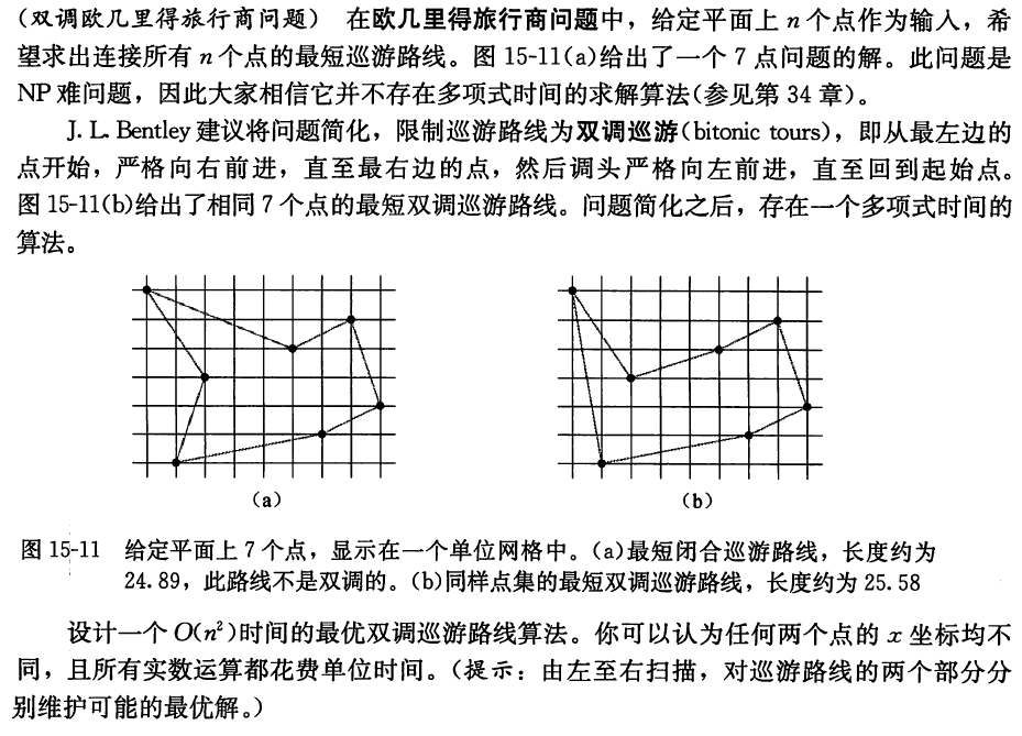
将 \(n\) 个点按 \(x\) 轴坐标进行排序, \(i(i = 1, 2, \cdots, n)\) 表示排序后第 \(i\) 个位置的坐标点
\(d[i, j]\) 表示第一条路线的终点为 \(i\), 第二条路线的终点为 \(j\) 时,巡游路线的最小值, 由于两条路线的对称性,不妨设 \(i \le j\)
\(j \gt 2\) 时,\(d[i, j]\) 可按以下递推式求得:
\(d[n, n]\) 的值即为最短路径
为了重构两条路径,需要维护另外一张表,\(k[1..n, 1..n]\),其中 \(k[i, i+1], i = 1, \cdots, n\) 表示 \(i == j-1\) 时所选择的最优的点 \(u\)
%%writefile ch15/bitonic_eucliden_travel.py
"""思考题15-3 双调欧几里得旅行商问题"""


def bitonic_euclidean_travel(coordinates):
  """应确保 coordinates 的 x 坐标按升序排列"""
  n = len(coordinates)
  p = [[ ((coordinates[i][0] - coordinates[j][0]) ** 2 + (coordinates[i][1] - coordinates[j][1]) ** 2)**0.5 if i < j else 0
        for j in range(n)]
        for i in range(n)]
  d = [[float(‘inf‘) if i == j-1 else 0
        for j in range(n)]
        for i in range(n)]
  d[0][0] = 0
  d[0][1] = p[0][1]
  d[1][1] = 2 * p[0][1]
  k = [[0]*n for i in range(n)]
  k[0][1] = 1
  for j in range(3, n+1):
    for i in range(1, j+1):
      if i == j - 1:
        for u in range(1, j-1):
          t = d[u-1][j-2] + p[u-1][j-1]
          if t < d[i-1][j-1]:
            d[i-1][j-1] = t
            k[i-1][j-1] = u
      elif i != j:
        d[i-1][j-1] = d[i-1][j-2] + p[j-2][j-1]
      else:
        d[i-1][j-1] = d[j-2][j-1] + p[j-2][j-1]
  # 重构解
  first, second = [], []
  i = n-1
  while i > 1:
    u = k[i-1][i]
    first.extend(reversed(range(u+1, i+1)))
    first, second = second, first
    i = u
  first = [coordinates[i-1] for i in first][::-1]
  second = [coordinates[i-1] for i in second][::-1]
  first.insert(0, coordinates[0])
  second.insert(0, coordinates[0])
  first.append(coordinates[-1])
  second.append(coordinates[-1])
  return d[-1][-1], first, second


if __name__ == "__main__":
  coordinates = ((0, 6), (1, 0), (2, 3), (5, 4), (6, 1), (7, 5), (8, 2))
  d, first, second = bitonic_euclidean_travel(coordinates)
  print("最短的双调欧几里得路径为:", d, "第一条路径为:", first, "第二条路径为:", second)
Overwriting ch15/bitonic_eucliden_travel.py
!python ch15/bitonic_eucliden_travel.py
最短的双调欧几里得路径为: 25.58402459469133 第一条路径为: [(0, 6), (2, 3), (5, 4), (7, 5), (8, 2)] 第二条路径为: [(0, 6), (1, 0), (6, 1), (8, 2)]
%%writefile ch15/printing_neatly.py
"""思考题 15-4 整齐打印"""


def printing_neatly(X, M):
  n = len(X)
  c = [0] * (n+1)
  b = [1] * n
  for j in range(1, n+1):
    c[j] = float(‘inf‘)
    blanks = M + 1  # 补上 i == j 时所减去的空格
    for i in reversed(range(1, j+1)):
      blanks -= 1 + len(X[i-1])
      if blanks < 0:
        break
      if j == n:  # 最后一个元素,无需加上最后一行
        if c[j-1] < c[j]:
          b[j-1] = i
          c[j] = c[j-1]
      else:
        t = c[i-1] + blanks ** 3
        if t < c[j]:
          b[j-1] = i
          c[j] = t

  # 重构最优解
  last_word = []  # 储存每一行最后一个单词对应的下标
  i = n
  while i > 0:
    last_word.append(i)
    i = b[i-1] - 1
  return c[n], last_word[::-1]


if __name__ == "__main__":
  s = """
  The Zen of Python, by Tim Peters

  Beautiful is better than ugly.
  Explicit is better than implicit.
  Simple is better than complex.
  Complex is better than complicated.
  Flat is better than nested.
  Sparse is better than dense.
  Readability counts.
  Special cases aren‘t special enough to break the rules.
  Although practicality beats purity.
  Errors should never pass silently.
  Unless explicitly silenced.
  In the face of ambiguity, refuse the temptation to guess.
  There should be one-- and preferably only one --obvious way to do it.
  Although that way may not be obvious at first unless you‘re Dutch.
  Now is better than never.
  Although never is often better than right now.
  If the implementation is hard to explain, it‘s a bad idea.
  If the implementation is easy to explain, it may be a good idea.
  Namespaces are one honking great idea -- let‘s do more of those1G!
  """.split()
  M = 80
  cost, last_word = printing_neatly(s, M)
  print("除最后一行外, 空格数立方的最小值之和为: ", cost)
  print("最终的打印结果为: ")
  print(‘*‘*80)
  for index, item in enumerate(last_word):
    if index == 0:
      print(" ".join(s[:item]).ljust(M, "|"))
    else:
      print(" ".join(s[last_word[index-1]:item]).ljust(M, "|"))
Overwriting ch15/printing_neatly.py
!python ch15/printing_neatly.py
除最后一行外, 空格数立方的最小值之和为:  1346
最终的打印结果为:
********************************************************************************
The Zen of Python, by Tim Peters Beautiful is better than ugly. Explicit||||||||
is better than implicit. Simple is better than complex. Complex is better|||||||
than complicated. Flat is better than nested. Sparse is better than dense.||||||
Readability counts. Special cases aren‘t special enough to break the rules.|||||
Although practicality beats purity. Errors should never pass silently. Unless|||
explicitly silenced. In the face of ambiguity, refuse the temptation to guess.||
There should be one-- and preferably only one --obvious way to do it. Although||
that way may not be obvious at first unless you‘re Dutch. Now is better than||||
never. Although never is often better than right now. If the implementation is||
hard to explain, it‘s a bad idea. If the implementation is easy to explain, it||
may be a good idea. Namespaces are one honking great idea -- let‘s do more of|||
those1G!||||||||||||||||||||||||||||||||||||||||||||||||||||||||||||||||||||||||
%%writefile ch15/edit_distance.py
"""思考题15-5 编辑距离"""


def edit_distance(x, y, cost):
  """求最小的编辑距离"""
  m, n = len(x), len(y)
  c = [[float(‘inf‘)]*(n+1) for i in range(m+1)]
  d = [[None]*(n+1) for i in range(m+1)]
  # 相关表项的初始化
  c[0][0] = 0
  for i in range(1, m+1):
    c[i][0] = i * cost[‘delete‘]
    d[i][0] = ‘delete‘
  for j in range(1, n+1):
    c[0][j] = j * cost[‘insert‘]
    d[0][j] = ‘insert‘
  for i in range(1, m+1):
    for j in range(1, n+1):
      if x[i-1] == y[j-1]:  # copy
        t = c[i-1][j-1] + cost[‘copy‘]
        if t < c[i][j]:
          c[i][j] = t
          d[i][j] = ‘copy‘
      else:  # replace
        t = c[i-1][j-1] + cost[‘replace‘]
        if t < c[i][j]:
          c[i][j] = t
          d[i][j] = ‘replace‘
      if i >= 2 and j >= 2 and x[i-1] == y[j-2] and x[i-2] == y[j-1]:  # twiddle
        t = c[i-2][j-2] + cost[‘twiddle‘]
        if t < c[i][j]:
          c[i][j] = t
          d[i][j] = ‘twiddle‘
      t = c[i-1][j] + cost[‘delete‘]  # delete
      if t < c[i][j]:
        c[i][j] = t
        d[i][j] = ‘delete‘
      t = c[i][j-1] + cost[‘insert‘]  # insert
      if t < c[i][j]:
        c[i][j] = t
        d[i][j] = ‘insert‘
  kill_index = -1
  for k in range(0, m):  # kill 操作
    t = c[k][n] + cost[‘kill‘]
    if t < c[m][n]:
      kill_index = k + 1
      c[m][n] = t
  # 重构最优解
  res = []
  if kill_index == -1:
    i, j = m, n
  else:
    i, j = kill_index, n
    res.append(‘kill‘)
  while i > 0 or j > 0:
    if d[i][j] == ‘copy‘:
      res.append(‘copy {}‘.format(x[i-1]))
      i, j = i-1, j-1
    elif d[i][j] == ‘replace‘:
      res.append(‘replace {} by {}‘.format(x[i-1], y[j-1]))
      i, j = i-1, j-1
    elif d[i][j] == ‘twiddle‘:
      res.append(‘twiddle {} with {}‘.format(x[i-1], x[i-2]))
      i, j = i-2, j-2
    elif d[i][j] == ‘delete‘:
      res.append(‘delete {}‘.format(x[i-1]))
      i = i - 1
    elif d[i][j] == ‘insert‘:
      res.append(‘insert {}‘.format(y[j-1]))
      j = j -1
  return c[m][n], res[::-1]
Writing ch15/edit_distance.py
import ch15.edit_distance
imp.reload(ch15.edit_distance)
from ch15.edit_distance import edit_distance
cost = dict(zip((‘copy‘, ‘replace‘, ‘delete‘, ‘insert‘, ‘twiddle‘, ‘kill‘), (1, 4, 2, 3, 2, 1)))
x, y = ‘algorithm‘, ‘altruistic‘
total_cost, res= edit_distance(x, y, cost)
print("编辑距离为:{}".format(total_cost), "操作过程为:", "\n".join(res), sep="\n")
编辑距离为:24
操作过程为:
copy a
copy l
delete g
replace o by t
copy r
insert u
insert i
insert s
twiddle t with i
replace h by c
kill
最优化对齐的最终目的可以等效于修改两个 DNA 序列,以让它们相同。插入操作相当于在 \(x\) 中插入空格,删除操作相当于在 \(y\) 中插入空格。
由“打分”规则可知,复制操作的代价为 \(1\), 替换操作的代价为 \(-1\), 插入和删除的代价为 \(-2\),算法的目的相当于是寻找最大编辑距离
根据插入和删除操作,分别向 \(x\), 与 \(y\) 中插入空格,即可构造出最优解
%%writefile -a ch15/edit_distance.py


def align_sequences(x, y, cost):
  """借助编辑距离求序列对齐的最佳方案"""
  m, n = len(x), len(y)
  c = [[float(‘-inf‘)]*(n+1) for i in range(m+1)]
  d = [[None]*(n+1) for i in range(m+1)]
  # 相关表项的初始化
  c[0][0] = 0
  for i in range(1, m+1):
    c[i][0] = i * cost[‘delete‘]
    d[i][0] = ‘delete‘
  for j in range(1, n+1):
    c[0][j] = j * cost[‘insert‘]
    d[0][j] = ‘insert‘
  for i in range(1, m+1):
    for j in range(1, n+1):
      if x[i-1] == y[j-1]:  # copy
        t = c[i-1][j-1] + cost[‘copy‘]
        if t > c[i][j]:
          c[i][j] = t
          d[i][j] = ‘copy‘
      else:  # replace
        t = c[i-1][j-1] + cost[‘replace‘]
        if t > c[i][j]:
          c[i][j] = t
          d[i][j] = ‘replace‘
      t = c[i-1][j] + cost[‘delete‘]  # delete
      if t > c[i][j]:
        c[i][j] = t
        d[i][j] = ‘delete‘
      t = c[i][j-1] + cost[‘insert‘]  # insert
      if t > c[i][j]:
        c[i][j] = t
        d[i][j] = ‘insert‘
  # 重构最优解
  i, j, x_blanks, y_blanks= m, n, [], []
  while i > 0 or j > 0:
    if d[i][j] == ‘copy‘:
      i, j = i-1, j-1
    elif d[i][j] == ‘replace‘:
      i, j = i-1, j-1
    elif d[i][j] == ‘delete‘:
      y_blanks.append(i-1)
      i = i - 1
    elif d[i][j] == ‘insert‘:
      x_blanks.append(j-1)
      j = j -1
  x_align, y_align = x, y
  for item in x_blanks:
    x_align = x_align[:item] + "*" + x_align[item:]
  for item in y_blanks:
    y_align = y_align[:item] + "*" + y_align[item:]

  return c[m][n], x_align, y_align
Appending to ch15/edit_distance.py
import ch15.edit_distance
imp.reload(ch15.edit_distance)
from ch15.edit_distance import align_sequences
cost = dict(zip((‘copy‘, ‘replace‘, ‘delete‘, ‘insert‘), (1, -1, -2, -2)))
x = "GATCGGCAT"
y = "CAATGTGAATC"
total_cost, x_align, y_align = align_sequences(x, y, cost)
print("最优对齐方案为:", x_align, y_align, sep="\n")
print("最优方案的分数为: ", total_cost)
最优对齐方案为:
*GATCGGCAT*
CAATGTGAATC
最优方案的分数为:  -3

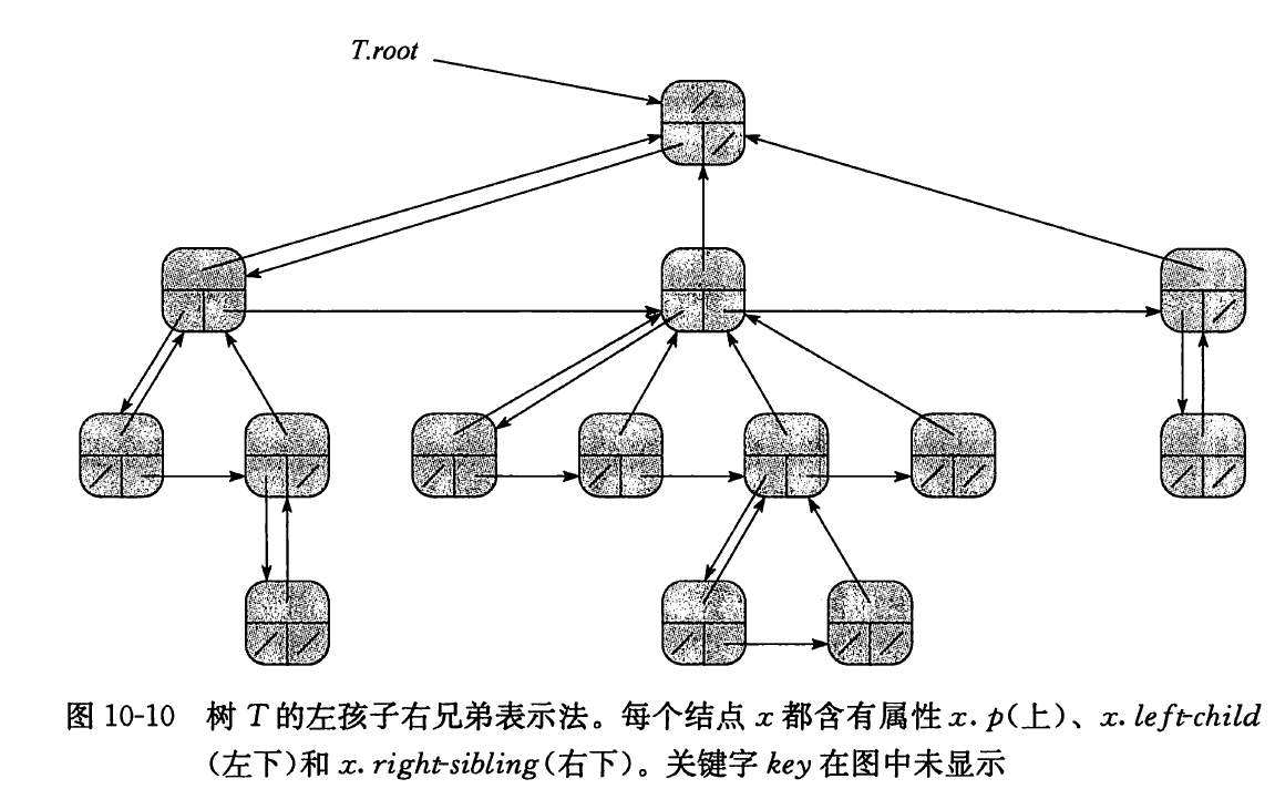
%%writefile ch15/party_plan.py
from collections import deque


class Node():
  """用来储存职员信息的结点"""
  def __init__(self, name=None, left_child=None, right_sibling=None, parent=None, point=0):
    self.name = name
    self.left_child = left_child
    self.right_sibling = right_sibling
    self.point = point
    self.parent = parent
    self.attend = None
    self.attend_points = None
    self.not_attend_points = None

  def __repr__(self):
    return str(self.name)

def calc_points(root):
  """计算特定结点的 attend_points 和 not_attend_points 属性"""
  if root.attend_points is not None:  # 避免重复计算
    return
  root.attend_points = root.point
  root.not_attend_points = 0
  child = root.left_child
  while child is not None:
    calc_points(child)
    root.attend_points += child.not_attend_points
    root.not_attend_points += max(child.attend_points, child.not_attend_points)
    child = child.right_sibling


def party_plan(root):
  """思考题 15-6 公司聚会计划"""
  calc_points(root)  # 自顶向下计算 attend_points 和 not_attend_points 属性
  # 层级遍历,构造出席人员
  res = []
  if root.attend_points > root.not_attend_points:
    root.attend, max_points = True, root.attend_points
    res.append(root)
  else:
    root.attend, max_points = False, root.not_attend_points
  if root.left_child is None:
    return max_points, res

  dq = deque()
  dq.append(root.left_child)
  while len(dq) > 0:
    x = dq.popleft()
    y = x
    while y is not None:
      if y.left_child is not None:
        dq.append(y.left_child)
      if y.parent.attend or y.attend_points < y.not_attend_points:
        y.attend = False
      else:
        y.attend = True
        res.append(y)
      y = y.right_sibling
  return max_points, res
Writing ch15/party_plan.py
import ch15.party_plan
imp.reload(ch15.party_plan)
from ch15.party_plan import Node, party_plan
points = [random.randint(1, 100) for i in range(14)]
N01 = Node(name=‘N01‘, point=points[0])
N11 = Node(name=‘N11‘, point=points[1])
N12 = Node(name=‘N12‘, point=points[2])
N13 = Node(name=‘N13‘, point=points[3])
N21 = Node(name=‘N21‘, point=points[4])
N22 = Node(name=‘N22‘, point=points[5])
N23 = Node(name=‘N23‘, point=points[6])
N24 = Node(name=‘N24‘, point=points[7])
N25 = Node(name=‘N25‘, point=points[8])
N26 = Node(name=‘N26‘, point=points[9])
N27 = Node(name=‘N27‘, point=points[10])
N31 = Node(name=‘N31‘, point=points[11])
N32 = Node(name=‘N32‘, point=points[12])
N33 = Node(name=‘N33‘, point=points[13])
N01.left_child = N11

N11.parent = N01
N12.parent = N01
N13.parent = N01
N11.right_sibling = N12
N12.right_sibling = N13
N11.left_child = N21
N12.left_child = N23
N13.left_child = N27

N21.parent = N11
N22.parent = N11
N21.right_sibling = N22
N22.left_child = N31

N23.parent = N12
N24.parent = N12
N25.parent = N12
N26.parent = N12
N23.right_sibling = N24
N24.right_sibling = N25
N25.right_sibling = N26
N25.left_child = N32

N27.parent = N13

N31.parent = N22

N32.parent = N25
N33.parent = N25
N32.right_sibling = N33
points
[38, 84, 11, 3, 14, 9, 86, 95, 34, 19, 46, 13, 82, 20]
max_points, res = party_plan(N01)
print("最高交际分数为:", max_points)
print("出席的人员为: ", ‘, ‘.join([str(item) for item in res]))
最高交际分数为: 445
出席的人员为:  N11, N23, N24, N26, N27, N31, N32, N33
与图算法相关,看完图的相关内容后再补
%%writefile ch15/seam_carving.py
def seam_carving(d):
  """思考题 15-8: 基于接链裁剪的图像压缩"""
  m, n = len(d), len(d[0])
  c = [[d[i][j] if i == 0 else 0 for j in range(n)] for i in range(m)]
  for i in range(1, m):
    c[i][0] = min(c[i-1][0], c[i-1][1]) + d[i][0]
    for j in range(1, n-1):
      c[i][j] = min(c[i-1][j-1], c[i-1][j] ,c[i-1][j+1]) + d[i][j]
    c[i][n-1] = min(c[i-1][n-2], c[i-1][n-1]) + d[i][j]

  # 重构最优解
  mini_cost, k = float(‘inf‘), None
  for i, item in enumerate(c[m-1]):
    if item < mini_cost:
      mini_cost, k = item, i
  res = [None] * m
  i = m - 1
  res[i] = (m, k+1)  # 储存剪切的位置

  for j in reversed(range(m-1)):
    mini_index = k
    if k != 0 and c[j][k-1] < c[j][mini_index]:
      mini_index = k - 1
    if k != n-1 and c[j][k+1] < c[j][mini_index]:
      mini_index = k + 1
    i -= 1
    res[i] = ((j+1, mini_index+1))
    k = mini_index
  return mini_cost, res


if __name__ == "__main__":
  import random

  d = [[random.randint(10, 99) for j in range(8)] for i in range(6)]
  print("破坏度矩阵为:")
  print("\n".join([str(item) for item in d]))
  mini_cost, res = seam_carving(d)
  print("最小破环度为: ", mini_cost)
  print("裁剪位置为:", res)
  res_sum = sum(d[item[0]-1][item[1]-1] for item in res)
  assert res_sum == mini_cost
Overwriting ch15/seam_carving.py
!python ch15/seam_carving.py
破坏度矩阵为:
[70, 67, 87, 57, 68, 74, 97, 81]
[41, 12, 74, 31, 21, 33, 44, 35]
[39, 26, 33, 13, 10, 33, 88, 44]
[17, 24, 40, 94, 38, 61, 33, 74]
[77, 99, 38, 75, 54, 44, 70, 24]
[59, 47, 68, 76, 86, 87, 62, 74]
最小破环度为:  214
裁剪位置为: [(1, 2), (2, 2), (3, 2), (4, 2), (5, 3), (6, 2)]
%%writefile ch15/string_break.py
def string_break(n, L):
  """思考题 15-9 字符串拆分"""
  m = len(L)
  L = [1] + list(L) + [n]
  c = [[L[j]-L[i] + 1 if j == i+2 else 1
      for j in range(m+2)]
      for i in range(m+2)]
  d = [[i+1 if j == i+2 else None
      for j in range(m+2)]
      for i in range(m+2)]
  for l in range(4, m+3):
    for i in range(0, m+3-l):
      j = i + l - 1
      c[i][j] = float(‘inf‘)
      for k in range(i+1, j):
        t = c[i][k] + c[k][j] + L[j] - L[i]
        if t < c[i][j]:
          c[i][j] = t
          d[i][j] = k

  mini_cost = c[0][m+1]  # 最小代价
  res = []
  construct_break_sequence(L, d, m, res, 0, m+1)
  return mini_cost, res


def construct_break_sequence(L, d, m, res, i, j):
  """构造最优拆分序列"""
  k = d[i][j]
  res.append(L[k])
  if k > i + 1:
    construct_break_sequence(L, d, m, res, i, k)
  if k < j - 1:
    construct_break_sequence(L, d, m, res, k, j)


if __name__ == "__main__":
  n = 20
  L = [2, 8, 10]
  mini_cost, res = string_break(n, L)
  print("最小拆分代价为:", mini_cost)
  print("对应的拆分序列为:", res)
Overwriting ch15/string_break.py
!python ch15/string_break.py
最小拆分代价为: 38
对应的拆分序列为: [10, 8, 2]
%%writefile ch15/invest_strategy.py
"""练习题 15-10: 投资策略规划"""


def invest_strategy(R, money, f1, f2):
  """R 储存了 n 种投资 m 年的收益"""
  n, m = len(R), len(R[0])
  c = [[money * R[i][0] if j == 0 else float(‘-inf‘)
      for j in range(m)]
      for i in range(n)]
  d = [[None]* (m) for i in range(n)]

  for j in range(1, m):
    for i in range(n):
      for k in range(n):
        if i == k:
          t = (c[k][j-1] - f1) * R[i][j]
        else:
          t = (c[k][j-1] - f2) * R[i][j]
        if t > c[i][j]:
          c[i][j] = t
          d[i][j] = k

  max_profit, k = float(‘-inf‘), None
  for i in range(n):
    if c[i][m-1] > max_profit:
      max_profit, k = c[i][m-1], i
  res = [None] * m
  res[-1] = k + 1
  for i in reversed(range(m-1)):
    res[i] = d[res[i+1] - 1][i+1] + 1
  return max_profit, res


if __name__ == "__main__":
  import numpy as np

  n, m = 5, 10
  R = np.random.random((n, m)) / 8 + 1
  money = 10 ** 4
  f1 = 50
  f2 = 500
  max_profit, res = invest_strategy(R, money, f1, f2)

  print("共有 {} 种投资, 投资年限为 {} 年".format(n, m))
  np.set_printoptions(precision=3, suppress=True, linewidth=100)
  print("每种投资的回报率为: \n", str(R))
  print("本金为: ", money)
  print("f1 = {}, f2 = {}".format(f1, f2))
  print("*"*50)
  print("最大收益为: ", max_profit)
  print("投资顺序为:", res)
Overwriting ch15/invest_strategy.py
!python ch15/invest_strategy.py
共有 5 种投资, 投资年限为 10 年
每种投资的回报率为:
 [[1.018 1.079 1.061 1.066 1.045 1.015 1.026 1.044 1.081 1.008]
 [1.04  1.087 1.068 1.041 1.053 1.09  1.105 1.089 1.102 1.014]
 [1.115 1.024 1.072 1.024 1.027 1.049 1.024 1.119 1.04  1.06 ]
 [1.052 1.072 1.025 1.093 1.032 1.11  1.032 1.067 1.045 1.042]
 [1.108 1.024 1.002 1.083 1.049 1.111 1.091 1.109 1.077 1.121]]
本金为:  10000
f1 = 50, f2 = 500
**************************************************
最大收益为:  21343.92608956265
投资顺序为: [3, 2, 2, 5, 5, 5, 5, 5, 5, 5]
%%writefile ch15/invest_strategy.py
"""思考题 15-11 库存规划"""
def invertory_plan(d):
  """库存规划
  """
  n, D = len(d), sum(d)
  c = [[ 0 if i == 0 else float(‘inf‘)
      for j in range(D+1)]
      for i in range(n+1)]
  b = [[0]*(D+1) for i in range(n+1)]
  w = [0]*(n+1)
  for i in range(1, n+1):
    w[i] = w[i-1] + d[i-1]
    for j in range(D-w[i]+1):
      c[i][j] = c[i-1][0] + product_cost(j+d[i-1]) + invertory_cost(j)
      if i == 1:
        continue
      for k in range(min(D-w[i-1], j+d[i-1])):
        t = c[i-1][k] + product_cost(j-k+d[i-1]) + invertory_cost(j)
        if t < c[i][j]:
          c[i][j] = t
          b[i][j] = k
  # 重构最优生产序列
  res, k = [0] * n, b[n][0]
  res[n-1] = -k+d[n-1]
  for i in reversed(range(i-1)):
    t = b[i+1][k]
    res[i] = k-t+d[i]
    k = t

  return c[n][0], res


def product_cost(x, m=10, c=1000):
  """生产成本`"""
  return 0 if x <=m else (x-m) * c


def invertory_cost(x):
  """存储成本"""
  return 250 * x


if __name__ == "__main__":
  import random
  d = [random.randint(0, 20) for i in range(11)] + [0]
  m, c = 10, 1000
  cost, res= invertory_plan(d)
  print("m = {}, c = {}".format(m, c))
  print("每件的储存成本为: 250")
  print("每个月销售量为:", d)
  print("*"*60)
  print("每个月的最优生产序列为: ", res)
  print("最低成本为: ", cost)
Overwriting ch15/invest_strategy.py
!python ch15/invest_strategy.py
m = 10, c = 1000
每件的储存成本为: 250
每个月销售量为: [10, 13, 3, 13, 10, 16, 14, 0, 19, 9, 3, 0]
************************************************************
每个月的最优生产序列为:  [10, 13, 10, 10, 10, 12, 14, 9, 10, 9, 3, 0]
最低成本为:  15000
%%writefile ch15/signing_players.py
"""思考题 15-2: 签约棒球自由球员"""


from collections import namedtuple

Player = namedtuple(‘Player‘, ‘index, cost, VORP‘)  # 球员属性, cost 的单位为十万


def signing_players(M, X):
  """M 应有 n 行 p 列,分别对应 N 个位置,以及每个位置上有 P 个可选球员"""
  N, P = len(M), len(M[0])
  x = X // 10 ** 5
  c = [[0]*(x+1) for i in range(N+1)]
  d = [[0]*(x+1) for i in range(N+1)]

  for i in range(1, N+1):
    for j in range(1, x+1):
      c[i][j] = float(‘-inf‘)
      if c[i-1][j] > c[i][j]:
        c[i][j], d[i][j] = c[i-1][j], 0
      for k in range(P):
        remain_money = j - M[i-1][k].cost
        if remain_money < 0:
          continue
        t = c[i-1][remain_money] + M[i-1][k].VORP
        if t > c[i][j]:
          c[i][j], d[i][j] = t, k+1

  # 重构最优解
  i, j, res = N, x, []
  while i > 0 and j > 0:
    k = d[i][j]
    if k != 0:
      res.append(M[i-1][k-1])
      i ,j = i-1, j - res[-1].cost
    else:
      i -= 1

  return c[N][x], res[::-1]


if __name__ == "__main__":
  import random
  N, P = 9, 6
  M = [[Player("{}{}".format(i+1, j+1), random.randint(1, 9), random.randint(60, 99))
      for j in range(P)]
      for i in range(N)]
  X = 12 * 10 ** 5
  print("球员信息为: \n")
  print("\n".join(str(item) for item in M))
  print("总的招聘费用为:{:.2f} 十万".format(X/10**5))
  print("*"*50)
  cost, res = signing_players(M, 12 * 10 ** 5)
  print("招入的球员为: ")
  print("\n".join(str(item) for item in res))
  print("最大 VORP 值为:", cost)
Overwriting ch15/signing_players.py
!python ch15/signing_players.py
球员信息为:

[Player(index=‘11‘, cost=5, VORP=62), Player(index=‘12‘, cost=9, VORP=75), Player(index=‘13‘, cost=8, VORP=83), Player(index=‘14‘, cost=3, VORP=91), Player(index=‘15‘, cost=2, VORP=86), Player(index=‘16‘, cost=6, VORP=74)]
[Player(index=‘21‘, cost=7, VORP=77), Player(index=‘22‘, cost=1, VORP=72), Player(index=‘23‘, cost=3, VORP=60), Player(index=‘24‘, cost=4, VORP=69), Player(index=‘25‘, cost=5, VORP=62), Player(index=‘26‘, cost=8, VORP=95)]
[Player(index=‘31‘, cost=6, VORP=78), Player(index=‘32‘, cost=8, VORP=83), Player(index=‘33‘, cost=8, VORP=93), Player(index=‘34‘, cost=7, VORP=62), Player(index=‘35‘, cost=7, VORP=97), Player(index=‘36‘, cost=2, VORP=80)]
[Player(index=‘41‘, cost=6, VORP=66), Player(index=‘42‘, cost=2, VORP=87), Player(index=‘43‘, cost=3, VORP=75), Player(index=‘44‘, cost=9, VORP=66), Player(index=‘45‘, cost=4, VORP=81), Player(index=‘46‘, cost=3, VORP=72)]
[Player(index=‘51‘, cost=9, VORP=75), Player(index=‘52‘, cost=3, VORP=60), Player(index=‘53‘, cost=1, VORP=66), Player(index=‘54‘, cost=3, VORP=73), Player(index=‘55‘, cost=2, VORP=82), Player(index=‘56‘, cost=3, VORP=95)]
[Player(index=‘61‘, cost=3, VORP=67), Player(index=‘62‘, cost=3, VORP=83), Player(index=‘63‘, cost=8, VORP=73), Player(index=‘64‘, cost=2, VORP=93), Player(index=‘65‘, cost=6, VORP=88), Player(index=‘66‘, cost=8, VORP=96)]
[Player(index=‘71‘, cost=6, VORP=70), Player(index=‘72‘, cost=2, VORP=88), Player(index=‘73‘, cost=7, VORP=70), Player(index=‘74‘, cost=4, VORP=85), Player(index=‘75‘, cost=4, VORP=97), Player(index=‘76‘, cost=3, VORP=66)]
[Player(index=‘81‘, cost=2, VORP=87), Player(index=‘82‘, cost=6, VORP=81), Player(index=‘83‘, cost=5, VORP=67), Player(index=‘84‘, cost=8, VORP=86), Player(index=‘85‘, cost=2, VORP=74), Player(index=‘86‘, cost=4, VORP=96)]
[Player(index=‘91‘, cost=5, VORP=95), Player(index=‘92‘, cost=3, VORP=68), Player(index=‘93‘, cost=9, VORP=79), Player(index=‘94‘, cost=4, VORP=86), Player(index=‘95‘, cost=4, VORP=74), Player(index=‘96‘, cost=6, VORP=96)]
总的招聘费用为:12.00 十万
**************************************************
招入的球员为:
Player(index=‘15‘, cost=2, VORP=86)
Player(index=‘22‘, cost=1, VORP=72)
Player(index=‘42‘, cost=2, VORP=87)
Player(index=‘53‘, cost=1, VORP=66)
Player(index=‘64‘, cost=2, VORP=93)
Player(index=‘72‘, cost=2, VORP=88)
Player(index=‘81‘, cost=2, VORP=87)
最大 VORP 值为: 579
标签:euc precision 限制 may 变量 形式 领域 多少 cbe
原文地址:https://www.cnblogs.com/lijunjie9502/p/12620013.html