标签:save 错误 parent 比例 return set nbsp post ram
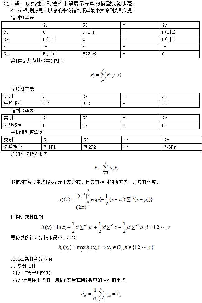
(1)掌握判别分析、主成分分析。
(2)会用判别分析、主成分分析对实际问题进行分析。
实验步骤要有模型建立,模型求解、结果分析。
(1)银行的贷款部门需要判别每个客户的信用好坏(是否未履行还贷责任),以决定是否给予贷款。可以根据贷款申请人的年龄(X1)、受教育程度(X2)、现在所从事工作的年数(X3)、未变更住址的年数(X4)、收入(X5)、负债收入比例(X6)、信用卡债务(X7)、其它债务(X8)等来判断其信用情况。下表是从某银行的客户资料中抽取的部分数据,和某客户的如上情况资料为(53,1,9,18,50,11.20,2.02,3.58),根据样本资料分别用马氏距离判别法、线性判别法、二次判别法对其进行信用好坏的判别。
|
目前信用好坏 |
客户序号 |
X1 |
X2 |
X3 |
X4 |
X5 |
X6 |
X7 |
X8 |
|
已履行还贷责任 |
1 |
23 |
1 |
7 |
2 |
31 |
6.60 |
0.34 |
1.71 |
|
2 |
34 |
1 |
17 |
3 |
59 |
8.00 |
1.81 |
2.91 |
|
|
3 |
42 |
2 |
7 |
23 |
41 |
4.60 |
0.94 |
.94 |
|
|
4 |
39 |
1 |
19 |
5 |
48 |
13.10 |
1.93 |
4.36 |
|
|
5 |
35 |
1 |
9 |
1 |
34 |
5.00 |
0.40 |
1.30 |
|
|
未履行还贷责任 |
6 |
37 |
1 |
1 |
3 |
24 |
15.10 |
1.80 |
1.82 |
|
7 |
29 |
1 |
13 |
1 |
42 |
7.40 |
1.46 |
1.65 |
|
|
8 |
32 |
2 |
11 |
6 |
75 |
23.30 |
7.76 |
9.72 |
|
|
9 |
28 |
2 |
2 |
3 |
23 |
6.40 |
0.19 |
1.29 |
|
|
10 |
26 |
1 |
4 |
3 |
27 |
10.50 |
2.47 |
.36 |
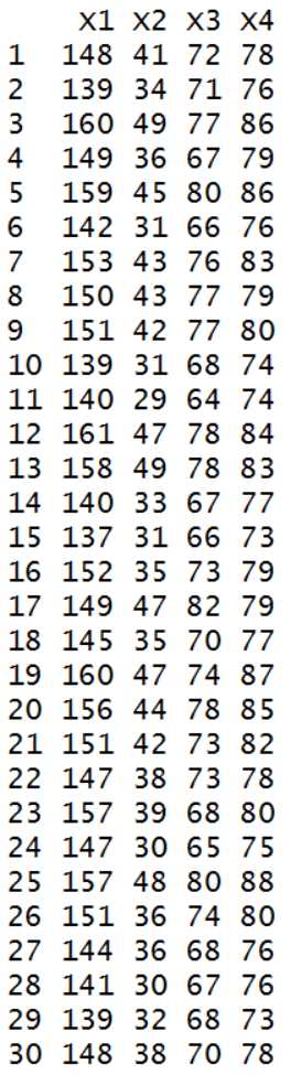
(2)在某中学随机抽取某年级30名学生,测量其身高(X1)、体重(X2)、胸围(X3)和坐高(X4),数据如表(30名中学生身体四项指标数据),试对这30名中学生身体四项指标数据做主成分分析。
|
组统计 |
|||||
|
group |
平均值 |
标准 偏差 |
有效个案数(成列) |
||
|
未加权 |
加权 |
||||
|
1.00 |
X1 |
34.6000 |
7.23187 |
5 |
5.000 |
|
X2 |
1.2000 |
.44721 |
5 |
5.000 |
|
|
X3 |
11.8000 |
5.76194 |
5 |
5.000 |
|
|
X4 |
6.8000 |
9.17606 |
5 |
5.000 |
|
|
X5 |
42.6000 |
11.28273 |
5 |
5.000 |
|
|
X6 |
7.4600 |
3.43045 |
5 |
5.000 |
|
|
X7 |
1.0840 |
.75580 |
5 |
5.000 |
|
|
X8 |
2.2440 |
1.39622 |
5 |
5.000 |
|
|
2.00 |
X1 |
30.4000 |
4.27785 |
5 |
5.000 |
|
X2 |
1.4000 |
.54772 |
5 |
5.000 |
|
|
X3 |
6.2000 |
5.44977 |
5 |
5.000 |
|
|
X4 |
3.2000 |
1.78885 |
5 |
5.000 |
|
|
X5 |
38.2000 |
21.94767 |
5 |
5.000 |
|
|
X6 |
12.5400 |
6.90312 |
5 |
5.000 |
|
|
X7 |
2.7360 |
2.92821 |
5 |
5.000 |
|
|
X8 |
2.9680 |
3.81647 |
5 |
5.000 |
|
|
总计 |
X1 |
32.5000 |
6.02310 |
10 |
10.000 |
|
X2 |
1.3000 |
.48305 |
10 |
10.000 |
|
|
X3 |
9.0000 |
6.05530 |
10 |
10.000 |
|
|
X4 |
5.0000 |
6.51494 |
10 |
10.000 |
|
|
X5 |
40.4000 |
16.61459 |
10 |
10.000 |
|
|
X6 |
10.0000 |
5.79463 |
10 |
10.000 |
|
|
X7 |
1.9100 |
2.19609 |
10 |
10.000 |
|
|
X8 |
2.6060 |
2.73598 |
10 |
10.000 |
|
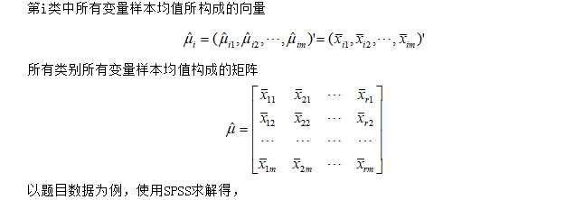
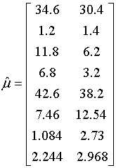
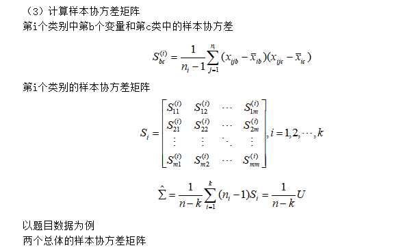
由上表得到下列式子:
|
协方差矩阵 |
|||||||||
|
group |
X1 |
X2 |
X3 |
X4 |
X5 |
X6 |
X7 |
X8 |
|
|
1.00 S1 |
X1 |
52.300 |
1.850 |
11.900 |
41.900 |
33.300 |
3.080 |
2.645 |
1.269 |
|
X2 |
1.850 |
.200 |
-1.200 |
4.050 |
-.400 |
-.715 |
-.036 |
-.326 |
|
|
X3 |
11.900 |
-1.200 |
33.200 |
-17.800 |
52.900 |
17.040 |
4.011 |
7.541 |
|
|
X4 |
41.900 |
4.050 |
-17.800 |
84.200 |
1.900 |
-10.035 |
.231 |
-4.857 |
|
|
X5 |
33.300 |
-.400 |
52.900 |
1.900 |
127.300 |
18.755 |
7.805 |
9.687 |
|
|
X6 |
3.080 |
-.715 |
17.040 |
-10.035 |
18.755 |
11.768 |
1.974 |
4.701 |
|
|
X7 |
2.645 |
-.036 |
4.011 |
.231 |
7.805 |
1.974 |
.571 |
.876 |
|
|
X8 |
1.269 |
-.326 |
7.541 |
-4.857 |
9.687 |
4.701 |
.876 |
1.949 |
|
|
2.00 S2 |
X1 |
18.300 |
-.200 |
-4.100 |
1.900 |
11.400 |
16.255 |
2.732 |
5.144 |
|
X2 |
-.200 |
.300 |
.150 |
.650 |
5.400 |
1.155 |
.620 |
1.269 |
|
|
X3 |
-4.100 |
.150 |
29.700 |
.200 |
91.200 |
8.415 |
7.896 |
10.551 |
|
|
X4 |
1.900 |
.650 |
.200 |
3.200 |
25.700 |
10.640 |
4.406 |
5.723 |
|
|
X5 |
11.400 |
5.400 |
91.200 |
25.700 |
481.700 |
114.065 |
58.751 |
78.620 |
|
|
X6 |
16.255 |
1.155 |
8.415 |
10.640 |
114.065 |
47.653 |
18.599 |
23.028 |
|
|
X7 |
2.732 |
.620 |
7.896 |
4.406 |
58.751 |
18.599 |
8.574 |
10.411 |
|
|
X8 |
5.144 |
1.269 |
10.551 |
5.723 |
78.620 |
23.028 |
10.411 |
14.565 |
|
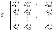
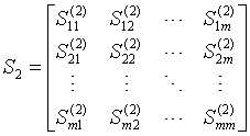
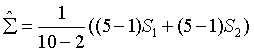
S1与S2见上表。
样本协方差矩阵由上表得到。
|
汇聚组内矩阵a |
|||||||||
|
|
X1 |
X2 |
X3 |
X4 |
X5 |
X6 |
X7 |
X8 |
|
|
协方差 |
X1 |
35.300 |
.825 |
3.900 |
21.900 |
22.350 |
9.668 |
2.688 |
3.206 |
|
X2 |
.825 |
.250 |
-.525 |
2.350 |
2.500 |
.220 |
.292 |
.471 |
|
|
X3 |
3.900 |
-.525 |
31.450 |
-8.800 |
72.050 |
12.728 |
5.953 |
9.046 |
|
|
X4 |
21.900 |
2.350 |
-8.800 |
43.700 |
13.800 |
.303 |
2.319 |
.433 |
|
|
X5 |
22.350 |
2.500 |
72.050 |
13.800 |
304.500 |
66.410 |
33.278 |
44.154 |
|
|
X6 |
9.668 |
.220 |
12.728 |
.303 |
66.410 |
29.711 |
10.287 |
13.864 |
|
|
X7 |
2.688 |
.292 |
5.953 |
2.319 |
33.278 |
10.287 |
4.573 |
5.644 |
|
|
X8 |
3.206 |
.471 |
9.046 |
.433 |
44.154 |
13.864 |
5.644 |
8.257 |
|
|
相关性 |
X1 |
1.000 |
.278 |
.117 |
.558 |
.216 |
.299 |
.212 |
.188 |
|
X2 |
.278 |
1.000 |
-.187 |
.711 |
.287 |
.081 |
.273 |
.328 |
|
|
X3 |
.117 |
-.187 |
1.000 |
-.237 |
.736 |
.416 |
.496 |
.561 |
|
|
X4 |
.558 |
.711 |
-.237 |
1.000 |
.120 |
.008 |
.164 |
.023 |
|
|
X5 |
.216 |
.287 |
.736 |
.120 |
1.000 |
.698 |
.892 |
.881 |
|
|
X6 |
.299 |
.081 |
.416 |
.008 |
.698 |
1.000 |
.883 |
.885 |
|
|
X7 |
.212 |
.273 |
.496 |
.164 |
.892 |
.883 |
1.000 |
.918 |
|
|
X8 |
.188 |
.328 |
.561 |
.023 |
.881 |
.885 |
.918 |
1.000 |
|
|
a. 协方差矩阵的自由度为 8。 |
|||||||||
|
分类函数系数 |
||
|
|
group |
|
|
1.00 |
2.00 |
|
|
X1 |
.340 |
.184 |
|
X2 |
94.070 |
126.660 |
|
X3 |
1.033 |
1.874 |
|
X4 |
-4.943 |
-6.681 |
|
X5 |
2.969 |
3.086 |
|
X6 |
13.723 |
17.182 |
|
X7 |
-10.994 |
-7.133 |
|
X8 |
-37.504 |
-49.116 |
|
(常量) |
-118.693 |
-171.296 |
|
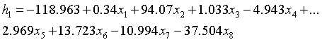
费希尔线性判别函数 |
||
第一类所对应的判别函数:
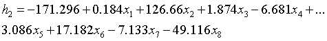
第二类所对应的判别函数:
3、判别效果验证,直接验证10个个体的原始数据
|
分类结果a |
|||||
|
|
|
group |
预测组成员信息 |
总计 |
|
|
|
|
1.00 |
2.00 |
||
|
原始 |
计数 |
1.00 |
5 |
0 |
5 |
|
2.00 |
0 |
5 |
5 |
||
|
未分组个案 |
1 |
0 |
1 |
||
|
% |
1.00 |
100.0 |
.0 |
100.0 |
|
|
2.00 |
.0 |
100.0 |
100.0 |
||
|
未分组个案 |
100.0 |
.0 |
100.0 |
||
|
a. 正确地对 100.0% 个原始已分组个案进行了分类。 |
|||||
第1类别的正确率100%;第2类别的正确类别100%。
最终结果,该客户为第1类“已履行还贷责任”。

代码:

1 DISCRIMINANT
2   /GROUPS=group(1 2)
3   /VARIABLES=X1 X2 X3 X4 X5 X6 X7 X8
4   /ANALYSIS ALL
5   /SAVE=CLASS SCORES PROBS
6   /PRIORS EQUAL
7   /STATISTICS=MEAN STDDEV UNIVF BOXM COEFF CORR COV GCOV TABLE
8   /CLASSIFY=NONMISSING POOLED.
马氏距离判别法和二次判别法的详细步骤依次类推,下面使用MATLAB编程应用马氏距离判别法,线性判别法和二次判别法求解题1。
MATLAB代码:
 1 % 样本数据
 2 training=[23,1,7,2,31,6.60,0.34,1.71
 3 34,1,17,3,59,8.00,1.81,2.91
 4 42,2,7,23,41,4.60,0.94,.94
 5 39,1,19,5,48,13.10,1.93,4.36
 6 35,1,9,1,34,5.00,0.40,1.30
 7 37,1,1,3,24,15.10,1.80,1.82
 8 29,1,13,1,42,7.40,1.46,1.65
 9 32,2,11,6,75,23.30,7.76,9.72
10 28,2,2,3,23,6.40,0.19,1.29
11 26,1,4,3,27,10.50,2.47,.36];
12 % 用于构造判别函数的样本数据矩阵
13 group=[1,1,1,1,1,2,2,2,2,2]‘;
14 % 参数group是与training相应的分组变量
15 sample=[53.00,1.00,9.00,18.00,50.00,11.20,2.02,3.58];
16 % 使用线性判别法分类
17 [class2,err2]=classify(sample,training,group,‘linear‘)
18 % 使用二次判别法分类
19 [class3,err3]=classify(sample,training,group,‘diagQuadratic‘)
20 % 使用马氏距离判别法分类
21 [class1,err1]=classify(sample,training,group,‘mahalanobis‘)
运行示例:
>> exp64
class2 =
1
err2 =
0
class3 =
1
err3 =
0.1000
错误使用 classify (line 282)
The covariance matrix of each group in TRAINING must be positive definite.
在运行过程中,二次判别这里使用的对角的二次判别代替基于协方差的二次判别;显然线性判别与上一步的求解结果一致,而二次判别与线性判别到结果都是把样本分类为第1类“已履行还贷责任”一类。但是在调用MATLAB的classify时,本题的数据使用马氏距离判别出现了协方差矩阵非正定的错误。(这个错误的来源并非是协方差,而是在求协方差矩阵的逆的时候有一些数据出现了过小的情况)
本报告修改classify代码如下:
1 %             if any(s <= max(gsize(k),d) * eps(max(s)))
2 %                 error(message(‘stats:classify:BadQuadVar‘));
3 %             end
完整代码:
  1 function [outclass, err, posterior, logp, coeffs] = classify(sample, training, group, type, prior)
  2 %CLASSIFY Discriminant analysis.
  3 %   CLASS = CLASSIFY(SAMPLE,TRAINING,GROUP) classifies each row of the data
  4 %   in SAMPLE into one of the groups in TRAINING.  SAMPLE and TRAINING must
  5 %   be matrices with the same number of columns.  GROUP is a grouping
  6 %   variable for TRAINING.  Its unique values define groups, and each
  7 %   element defines which group the corresponding row of TRAINING belongs
  8 %   to.  GROUP can be a categorical variable, numeric vector, a string
  9 %   array, or a cell array of strings.  TRAINING and GROUP must have the
 10 %   same number of rows.  CLASSIFY treats NaNs or empty strings in GROUP as
 11 %   missing values, and ignores the corresponding rows of TRAINING. CLASS
 12 %   indicates which group each row of SAMPLE has been assigned to, and is
 13 %   of the same type as GROUP.
 14 %
 15 %   CLASS = CLASSIFY(SAMPLE,TRAINING,GROUP,TYPE) allows you to specify the
 16 %   type of discriminant function, one of ‘linear‘, ‘quadratic‘,
 17 %   ‘diagLinear‘, ‘diagQuadratic‘, or ‘mahalanobis‘.  Linear discrimination
 18 %   fits a multivariate normal density to each group, with a pooled
 19 %   estimate of covariance.  Quadratic discrimination fits MVN densities
 20 %   with covariance estimates stratified by group.  Both methods use
 21 %   likelihood ratios to assign observations to groups.  ‘diagLinear‘ and
 22 %   ‘diagQuadratic‘ are similar to ‘linear‘ and ‘quadratic‘, but with
 23 %   diagonal covariance matrix estimates.  These diagonal choices are
 24 %   examples of naive Bayes classifiers.  Mahalanobis discrimination uses
 25 %   Mahalanobis distances with stratified covariance estimates.  TYPE
 26 %   defaults to ‘linear‘.
 27 %
 28 %   CLASS = CLASSIFY(SAMPLE,TRAINING,GROUP,TYPE,PRIOR) allows you to
 29 %   specify prior probabilities for the groups in one of three ways.  PRIOR
 30 %   can be a numeric vector of the same length as the number of unique
 31 %   values in GROUP (or the number of levels defined for GROUP, if GROUP is
 32 %   categorical).  If GROUP is numeric or categorical, the order of PRIOR
 33 %   must correspond to the ordered values in GROUP, or, if GROUP contains
 34 %   strings, to the order of first occurrence of the values in GROUP. PRIOR
 35 %   can also be a 1-by-1 structure with fields ‘prob‘, a numeric vector,
 36 %   and ‘group‘, of the same type as GROUP, and containing unique values
 37 %   indicating which groups the elements of ‘prob‘ correspond to. As a
 38 %   structure, PRIOR may contain groups that do not appear in GROUP. This
 39 %   can be useful if TRAINING is a subset of a larger training set.
 40 %   CLASSIFY ignores any groups that appear in the structure but not in the
 41 %   GROUPS array.  Finally, PRIOR can also be the string value ‘empirical‘,
 42 %   indicating that the group prior probabilities should be estimated from
 43 %   the group relative frequencies in TRAINING.  PRIOR defaults to a
 44 %   numeric vector of equal probabilities, i.e., a uniform distribution.
 45 %   PRIOR is not used for discrimination by Mahalanobis distance, except
 46 %   for error rate calculation.
 47 %
 48 %   [CLASS,ERR] = CLASSIFY(...) returns ERR, an estimate of the
 49 %   misclassification error rate that is based on the training data.
 50 %   CLASSIFY returns the apparent error rate, i.e., the percentage of
 51 %   observations in the TRAINING that are misclassified, weighted by the
 52 %   prior probabilities for the groups.
 53 %
 54 %   [CLASS,ERR,POSTERIOR] = CLASSIFY(...) returns POSTERIOR, a matrix
 55 %   containing estimates of the posterior probabilities that the j‘th
 56 %   training group was the source of the i‘th sample observation, i.e.
 57 %   Pr{group j | obs i}.  POSTERIOR is not computed for Mahalanobis
 58 %   discrimination.
 59 %
 60 %   [CLASS,ERR,POSTERIOR,LOGP] = CLASSIFY(...) returns LOGP, a vector
 61 %   containing estimates of the logs of the unconditional predictive
 62 %   probability density of the sample observations, p(obs i) is the sum of
 63 %   p(obs i | group j)*Pr{group j} taken over all groups.  LOGP is not
 64 %   computed for Mahalanobis discrimination.
 65 %
 66 %   [CLASS,ERR,POSTERIOR,LOGP,COEF] = CLASSIFY(...) returns COEF, a
 67 %   structure array containing coefficients describing the boundary between
 68 %   the regions separating each pair of groups.  Each element COEF(I,J)
 69 %   contains information for comparing group I to group J, defined using
 70 %   the following fields:
 71 %       ‘type‘      type of discriminant function, from TYPE input
 72 %       ‘name1‘     name of first group of pair (group I)
 73 %       ‘name2‘     name of second group of pair (group J)
 74 %       ‘const‘     constant term of boundary equation (K)
 75 %       ‘linear‘    coefficients of linear term of boundary equation (L)
 76 %       ‘quadratic‘ coefficient matrix of quadratic terms (Q)
 77 %
 78 %   For the ‘linear‘ and ‘diaglinear‘ types, the ‘quadratic‘ field is
 79 %   absent, and a row x from the SAMPLE array is classified into group I
 80 %   rather than group J if
 81 %         0 < K + x*L
 82 %   For the other types, x is classified into group I if
 83 %         0 < K + x*L + x*Q*x‘
 84 %
 85 %   Example:
 86 %      % Classify Fisher iris data using quadratic discriminant function
 87 %      load fisheriris
 88 %      x = meas(51:end,1:2);  % for illustrations use 2 species, 2 columns
 89 %      y = species(51:end);
 90 %      [c,err,post,logl,str] = classify(x,x,y,‘quadratic‘);
 91 %      h = gscatter(x(:,1),x(:,2),y,‘rb‘,‘v^‘);
 92 %
 93 %      % Classify a grid of values
 94 %      [X,Y] = meshgrid(linspace(4.3,7.9), linspace(2,4.4));
 95 %      X = X(:); Y = Y(:);
 96 %      C = classify([X Y],x,y,‘quadratic‘);
 97 %      hold on; gscatter(X,Y,C,‘rb‘,‘.‘,1,‘off‘); hold off
 98 %
 99 %      % Draw boundary between two regions
100 %      hold on
101 %      K = str(1,2).const;
102 %      L = str(1,2).linear;
103 %      Q = str(1,2).quadratic;
104 %      % Plot the curve K + [x,y]*L + [x,y]*Q*[x,y]‘ = 0:
105 %      f = @(x,y) K + L(1)*x + L(2)*y ...
106 %                   + Q(1,1)*x.^2 + (Q(1,2)+Q(2,1))*x.*y + Q(2,2)*y.^2;
107 %      ezplot(f,[4 8 2 4.5]);
108 %      hold off
109 %      title(‘Classification of Fisher iris data‘)
110 %      legend(h)
111 %
112 %   See also fitcdiscr, fitcnb.
113
114 %   Copyright 1993-2018 The MathWorks, Inc.
115
116
117 %   References:
118 %     [1] Krzanowski, W.J., Principles of Multivariate Analysis,
119 %         Oxford University Press, Oxford, 1988.
120 %     [2] Seber, G.A.F., Multivariate Observations, Wiley, New York, 1984.
121
122 if nargin < 3
123     error(message(‘stats:classify:TooFewInputs‘));
124 end
125
126 if nargin>3
127     type = convertStringsToChars(type);
128 end
129
130 % grp2idx sorts a numeric grouping var ascending, and a string grouping
131 % var by order of first occurrence
132 [gindex,groups,glevels] = grp2idx(group);
133 nans = find(isnan(gindex));
134 if ~isempty(nans)
135     training(nans,:) = [];
136     gindex(nans) = [];
137 end
138 ngroups = length(groups);
139 gsize = hist(gindex,1:ngroups);
140 nonemptygroups = find(gsize>0);
141 nusedgroups = length(nonemptygroups);
142 if ngroups > nusedgroups
143     warning(message(‘stats:classify:EmptyGroups‘));
144
145 end
146
147 [n,d] = size(training);
148 if size(gindex,1) ~= n
149     error(message(‘stats:classify:TrGrpSizeMismatch‘));
150 elseif isempty(sample)
151     sample = zeros(0,d,class(sample));  % accept any empty array but force correct size
152 elseif size(sample,2) ~= d
153     error(message(‘stats:classify:SampleTrColSizeMismatch‘));
154 end
155 m = size(sample,1);
156
157 if nargin < 4 || isempty(type)
158     type = ‘linear‘;
159 elseif ischar(type)
160     types = {‘linear‘,‘quadratic‘,‘diaglinear‘,‘diagquadratic‘,‘mahalanobis‘};
161     type = internal.stats.getParamVal(type,types,‘TYPE‘);
162 else
163     error(message(‘stats:classify:BadType‘));
164 end
165
166 % Default to a uniform prior
167 if nargin < 5 || isempty(prior)
168     prior = ones(1, ngroups) / nusedgroups;
169     prior(gsize==0) = 0;
170     % Estimate prior from relative group sizes
171 elseif ischar(prior) && strncmpi(prior,‘empirical‘,length(prior))
172     %~isempty(strmatch(lower(prior), ‘empirical‘))
173     prior = gsize(:)‘ / sum(gsize);
174     % Explicit prior
175 elseif isnumeric(prior)
176     if min(size(prior)) ~= 1 || max(size(prior)) ~= ngroups
177         error(message(‘stats:classify:GrpPriorSizeMismatch‘));
178     elseif any(prior < 0)
179         error(message(‘stats:classify:BadPrior‘));
180     end
181     %drop empty groups
182     prior(gsize==0)=0;
183     prior = prior(:)‘ / sum(prior); % force a normalized row vector
184 elseif isstruct(prior)
185     [pgindex,pgroups] = grp2idx(prior.group);
186
187     ord = NaN(1,ngroups);
188     for i = 1:ngroups
189       j = find(strcmp(groups(i), pgroups(pgindex)));
190         if ~isempty(j)
191             ord(i) = j;
192         end
193     end
194     if any(isnan(ord))
195         error(message(‘stats:classify:PriorBadGrpup‘));
196     end
197     prior = prior.prob(ord);
198     if any(prior < 0)
199         error(message(‘stats:classify:PriorBadProb‘));
200     end
201     prior(gsize==0)=0;
202     prior = prior(:)‘ / sum(prior); % force a normalized row vector
203 else
204     error(message(‘stats:classify:BadPriorType‘));
205 end
206
207 % Add training data to sample for error rate estimation
208 if nargout > 1
209     sample = [sample; training];
210     mm = m+n;
211 else
212     mm = m;
213 end
214
215 gmeans = NaN(ngroups, d);
216 for k = nonemptygroups
217     gmeans(k,:) = mean(training(gindex==k,:),1);
218 end
219
220 D = NaN(mm, ngroups);
221 isquadratic = false;
222 switch type
223     case ‘linear‘
224         if n <= nusedgroups
225             error(message(‘stats:classify:NTrainingTooSmall‘));
226         end
227         % Pooled estimate of covariance.  Do not do pivoting, so that A can be
228         % computed without unpermuting.  Instead use SVD to find rank of R.
229         [Q,R] = qr(training - gmeans(gindex,:), 0);
230         R = R / sqrt(n - nusedgroups); % SigmaHat = R‘*R
231         s = svd(R);
232         if any(s <= max(n,d) * eps(max(s)))
233             error(message(‘stats:classify:BadLinearVar‘));
234         end
235         logDetSigma = 2*sum(log(s)); % avoid over/underflow
236
237         % MVN relative log posterior density, by group, for each sample
238         for k = nonemptygroups
239             A = bsxfun(@minus,sample, gmeans(k,:)) / R;
240             D(:,k) = log(prior(k)) - .5*(sum(A .* A, 2) + logDetSigma);
241         end
242
243     case ‘diaglinear‘
244         if n <= nusedgroups
245             error(message(‘stats:classify:NTrainingTooSmall‘));
246         end
247         % Pooled estimate of variance: SigmaHat = diag(S.^2)
248         S = std(training - gmeans(gindex,:)) * sqrt((n-1)./(n-nusedgroups));
249
250         if any(S <= n * eps(max(S)))
251             error(message(‘stats:classify:BadDiagLinearVar‘));
252         end
253         logDetSigma = 2*sum(log(S)); % avoid over/underflow
254
255         if nargout >= 5
256             R = S‘;
257         end
258
259         % MVN relative log posterior density, by group, for each sample
260         for k = nonemptygroups
261             A=bsxfun(@times, bsxfun(@minus,sample,gmeans(k,:)),1./S);
262             D(:,k) = log(prior(k)) - .5*(sum(A .* A, 2) + logDetSigma);
263         end
264
265     case {‘quadratic‘ ‘mahalanobis‘}
266         if any(gsize == 1)
267             error(message(‘stats:classify:BadTraining‘));
268         end
269         isquadratic = true;
270         logDetSigma = zeros(ngroups,1,class(training));
271         if nargout >= 5
272           R = zeros(d,d,ngroups,class(training));
273         end
274         for k = nonemptygroups
275             % Stratified estimate of covariance.  Do not do pivoting, so that A
276             % can be computed without unpermuting.  Instead use SVD to find rank
277             % of R.
278             [Q,Rk] = qr(bsxfun(@minus,training(gindex==k,:),gmeans(k,:)), 0);
279             Rk = Rk / sqrt(gsize(k) - 1); % SigmaHat = R‘*R
280             s = svd(Rk);
281 %             if any(s <= max(gsize(k),d) * eps(max(s)))
282 %                 error(message(‘stats:classify:BadQuadVar‘));
283 %             end
284             logDetSigma(k) = 2*sum(log(s)); % avoid over/underflow
285
286             A = bsxfun(@minus, sample, gmeans(k,:)) /Rk;
287             switch type
288                 case ‘quadratic‘
289                     % MVN relative log posterior density, by group, for each sample
290                     D(:,k) = log(prior(k)) - .5*(sum(A .* A, 2) + logDetSigma(k));
291                 case ‘mahalanobis‘
292                     % Negative squared Mahalanobis distance, by group, for each
293                     % sample.  Prior probabilities are not used
294                     D(:,k) = -sum(A .* A, 2);
295             end
296             if nargout >=5 && ~isempty(Rk)
297                 R(:,:,k) = inv(Rk);
298             end
299         end
300
301     case ‘diagquadratic‘
302         if any(gsize == 1)
303             error(message(‘stats:classify:BadTraining‘));
304         end
305         isquadratic = true;
306         logDetSigma = zeros(ngroups,1,class(training));
307         if nargout >= 5
308             R = zeros(d,1,ngroups,class(training));
309         end
310         for k = nonemptygroups
311             % Stratified estimate of variance:  SigmaHat = diag(S.^2)
312             S = std(training(gindex==k,:));
313             if any(S <= gsize(k) * eps(max(S)))
314                 error(message(‘stats:classify:BadDiagQuadVar‘));
315             end
316             logDetSigma(k) = 2*sum(log(S)); % avoid over/underflow
317
318             % MVN relative log posterior density, by group, for each sample
319             A=bsxfun(@times, bsxfun(@minus,sample,gmeans(k,:)),1./S);
320             D(:,k) = log(prior(k)) - .5*(sum(A .* A, 2) + logDetSigma(k));
321             if nargout >= 5
322               R(:,:,k) = 1./S‘;
323             end
324         end
325 end
326
327 % find nearest group to each observation in sample data
328 [maxD,outclass] = max(D, [], 2);
329
330 % Compute apparent error rate: percentage of training data that
331 % are misclassified, weighted by the prior probabilities for the groups.
332 if nargout > 1
333     trclass = outclass(m+(1:n));
334     outclass = outclass(1:m);
335
336     miss = trclass ~= gindex;
337     e = zeros(ngroups,1);
338     for k = nonemptygroups
339         e(k) = sum(miss(gindex==k)) / gsize(k);
340     end
341     err = prior*e;
342 end
343
344 if nargout > 2
345     if strcmp(type, ‘mahalanobis‘)
346         % Mahalanobis discrimination does not use the densities, so it‘s
347         % possible that the posterior probs could disagree with the
348         % classification.
349         posterior = [];
350         logp = [];
351     else
352         % Bayes‘ rule: first compute p{x,G_j} = p{x|G_j}Pr{G_j} ...
353         % (scaled by max(p{x,G_j}) to avoid over/underflow)
354         P = exp(bsxfun(@minus,D(1:m,:),maxD(1:m)));
355         sumP = nansum(P,2);
356         % ... then Pr{G_j|x) = p(x,G_j} / sum(p(x,G_j}) ...
357         % (numer and denom are both scaled, so it cancels out)
358         posterior = bsxfun(@times,P,1./(sumP));
359         if nargout > 3
360             % ... and unconditional p(x) = sum(p(x,G_j}).
361             % (remove the scale factor)
362             logp = log(sumP) + maxD(1:m) - .5*d*log(2*pi);
363         end
364     end
365 end
366
367 %Convert outclass back to original grouping variable type
368  outclass = glevels(outclass,:);
369
370 if nargout>=5
371     pairs = combnk(nonemptygroups,2)‘;
372     npairs = size(pairs,2);
373     K = zeros(1,npairs,class(training));
374     L = zeros(d,npairs,class(training));
375     if ~isquadratic
376         % Methods with equal covariances across groups
377         for j=1:npairs
378             % Compute const (K) and linear (L) coefficients for
379             % discriminating between each pair of groups
380             i1 = pairs(1,j);
381             i2 = pairs(2,j);
382             mu1 = gmeans(i1,:)‘;
383             mu2 = gmeans(i2,:)‘;
384             if ~strcmp(type,‘diaglinear‘)
385                 b = R \ ((R‘) \ (mu1 - mu2));
386             else
387                 b = (1./R).^2 .*(mu1 -mu2);
388             end
389             L(:,j) = b;
390             K(j) = 0.5 * (mu1 + mu2)‘ * b;
391         end
392     else
393         % Methods with separate covariances for each group
394         Q = zeros(d,d,npairs,class(training));
395         for j=1:npairs
396             % As above, but compute quadratic (Q) coefficients as well
397             i1 = pairs(1,j);
398             i2 = pairs(2,j);
399             mu1 = gmeans(i1,:)‘;
400             mu2 = gmeans(i2,:)‘;
401             R1i = R(:,:,i1);    % note here the R array contains inverses
402             R2i = R(:,:,i2);
403             if ~strcmp(type,‘diagquadratic‘)
404                 Rm1 = R1i‘ * mu1;
405                 Rm2 = R2i‘ * mu2;
406             else
407                 Rm1 = R1i .* mu1;
408                 Rm2 = R2i .* mu2;
409             end
410             K(j) = 0.5 * (sum(Rm1.^2) - sum(Rm2.^2));
411             if ~strcmp(type, ‘mahalanobis‘)
412                 K(j) = K(j) + 0.5 * (logDetSigma(i1)-logDetSigma(i2));
413             end
414             if ~strcmp(type,‘diagquadratic‘)
415                 L(:,j) = (R1i*Rm1 - R2i*Rm2);
416                 Q(:,:,j) = -0.5 * (R1i*R1i‘ - R2i*R2i‘);
417             else
418                 L(:,j) = (R1i.*Rm1 - R2i.*Rm2);
419                 Q(:,:,j) = -0.5 * diag(R1i.^2 - R2i.^2);
420             end
421         end
422     end
423
424     % For all except Mahalanobis, adjust for the priors
425     if ~strcmp(type, ‘mahalanobis‘)
426         K = K - log(prior(pairs(1,:))) + log(prior(pairs(2,:)));
427     end
428
429     % Return information as a structure
430     coeffs = struct(‘type‘,repmat({type},ngroups,ngroups));
431     for k=1:npairs
432         i = pairs(1,k);
433         j = pairs(2,k);
434         coeffs(i,j).name1 = glevels(i,:);
435         coeffs(i,j).name2 = glevels(j,:);
436         coeffs(i,j).const = -K(k);
437         coeffs(i,j).linear = L(:,k);
438
439         coeffs(j,i).name1 = glevels(j,:);
440         coeffs(j,i).name2 = glevels(i,:);
441         coeffs(j,i).const = K(k);
442         coeffs(j,i).linear = -L(:,k);
443
444         if isquadratic
445             coeffs(i,j).quadratic = Q(:,:,k);
446             coeffs(j,i).quadratic = -Q(:,:,k);
447         end
448     end
449 end
运行代码:
 1 % 样本数据
 2 training=[23,1,7,2,31,6.60,0.34,1.71
 3 34,1,17,3,59,8.00,1.81,2.91
 4 42,2,7,23,41,4.60,0.94,.94
 5 39,1,19,5,48,13.10,1.93,4.36
 6 35,1,9,1,34,5.00,0.40,1.30
 7 37,1,1,3,24,15.10,1.80,1.82
 8 29,1,13,1,42,7.40,1.46,1.65
 9 32,2,11,6,75,23.30,7.76,9.72
10 28,2,2,3,23,6.40,0.19,1.29
11 26,1,4,3,27,10.50,2.47,.36];
12 % 用于构造判别函数的样本数据矩阵
13 group=[1,1,1,1,1,2,2,2,2,2]‘;
14 % 参数group是与training相应的分组变量
15 sample=[53.00,1.00,9.00,18.00,50.00,11.20,2.02,3.58];
16 % 使用线性判别法分类
17 [class2,err2]=classify(sample,training,group,‘linear‘)
18 % 使用马氏距离判别法分类
19 [class1,err1]=classify(sample,training,group,‘mahalanobis‘)
20 % 使用二次判别法分类
21 [class3,err3]=classify(sample,training,group,‘quadratic‘)
运行示例:
>> exp64
class2 =
1
err2 =
0
警告: 秩亏,秩 = 4,tol = 1.864663e-14。
> In classify (line 286)
In exp64 (line 19)
警告: 秩亏,秩 = 4,tol = 3.243458e-14。
> In classify (line 286)
In exp64 (line 19)
class1 =
1
err1 =
0.2000
警告: 秩亏,秩 = 4,tol = 1.864663e-14。
> In classify (line 286)
In exp64 (line 21)
警告: 秩亏,秩 = 4,tol = 3.243458e-14。
> In classify (line 286)
In exp64 (line 21)
class3 =
1
err3 =
0.2000
显然,线性判别、二次判别和马氏距离判别都把样本归为第1类“已履行还贷责任”。那么最终结果该贷款人是已履行还贷责任一类。这里,因为在第二步MATLAB运行过程中,出现警告,这里本报告手写一份马氏距离判别的程序以作验证,二次判别以此类推。函数代码:
 1 % 马氏距离判别
 2 % 输入:G1组别1,G2组别2,待分类x
 3 % 输出:分类序号
 4 function w=ma(G1,G2,x)
 5 [n1,m1]=size(G1);
 6 [n2,m2]=size(G2);
 7 if m1~=m2
 8     error(‘两个样本的列数应该相等!!‘);
 9 end
10 [n,~]=size(x);
11 w=zeros(n,1);
12 % 协方差
13 g1=cov(G1)./(n1-1);
14 g2=cov(G2)./(n2-1);
15 % 参数估计
16 for i=1:m1
17     niu1(i)=mean(G1(:,i));
18 end
19 for i=1:m2
20     niu2(i)=mean(G2(:,i));
21 end
22 % 马氏距离求解
23 v1=inv(g1);
24 v2=inv(g2);
25 d1=(x-niu1)‘.*v1.*(x-niu1);
26 d2=(x-niu2)‘.*v2.*(x-niu2);
27 k=1;
28 for j=1:n
29     if det(d1)>det(d2)
30         w(k)=2;
31         k=k+1;
32     else
33         w(k)=1;
34         k=k+1;
35     end
36 end
37 end
运行代码:
 1 G1=[23,1,7,2,31,6.60,0.34,1.71
 2 34,1,17,3,59,8.00,1.81,2.91
 3 42,2,7,23,41,4.60,0.94,.94
 4 39,1,19,5,48,13.10,1.93,4.36
 5 35,1,9,1,34,5.00,0.40,1.30];
 6 G2=[37,1,1,3,24,15.10,1.80,1.82
 7 29,1,13,1,42,7.40,1.46,1.65
 8 32,2,11,6,75,23.30,7.76,9.72
 9 28,2,2,3,23,6.40,0.19,1.29
10 26,1,4,3,27,10.50,2.47,.36];
11 x=[53.00,1.00,9.00,18.00,50.00,11.20,2.02,3.58];
12 w=ma(G1,G2,x)
运行示例:
>> exp64
警告: 矩阵接近奇异值,或者缩放错误。结果可能不准确。RCOND = 2.592596e-20。
> In ma (line 23)
In exp64 (line 44)
警告: 矩阵接近奇异值,或者缩放错误。结果可能不准确。RCOND = 1.123714e-19。
> In ma (line 24)
In exp64 (line 44)
w =
1
明显,手写的马氏距离代码运行结果同样把样本归为第1类“已履行还贷责任”。但是,同样在手写的代码中同样有与classify相似的警告,从这次警告可以知道警告出现在协方差矩阵的逆接近奇异值。(并非是因为正定性的原因,之所以判断为非正定是因为值太小,被计算机认为等于0)
因此可以放大协方差矩阵的逆矩阵,已通过未修改的classify函数。这里不予详细展示。基于“一个半正定阵加一个正定阵就会成为一个正定阵”的思想,这里对手写的马氏距离判别代码作出如下修改:(原矩阵+一个1e-4的单位阵,当然可以更小,这里不予论证!)
 1 % 马氏距离判别
 2 % 输入:G1组别1,G2组别2,待分类x
 3 % 输出:分类序号
 4 function w=ma(G1,G2,x)
 5 [n1,m1]=size(G1);
 6 [n2,m2]=size(G2);
 7 if m1~=m2
 8     error(‘两个样本的列数应该相等!!‘);
 9 end
10 [n,~]=size(x);
11 w=zeros(n,1);
12 % 协方差
13 g1=cov(G1)./(n1-1);
14 g2=cov(G2)./(n2-1);
15 [t1,t2]=size(g1);
16 g1=g1+eye(t1,t2)*1e-4;%修
17 g2=g2+eye(t1,t2)*1e-4;%修
18 % 参数估计
19 for i=1:m1
20     niu1(i)=mean(G1(:,i));
21 end
22 for i=1:m2
23     niu2(i)=mean(G2(:,i));
24 end
25 % 马氏距离求解
26 v1=inv(g1);
27 v2=inv(g2);
28 d1=(x-niu1)‘.*v1.*(x-niu1);
29 d2=(x-niu2)‘.*v2.*(x-niu2);
30 k=1;
31 for j=1:n
32     if det(d1)>det(d2)
33         w(k)=2;
34         k=k+1;
35     else
36         w(k)=1;
37         k=k+1;
38     end
39 end
40 end
运行效果:
>> exp64
w =
1
如此,解决了奇异值的问题。那么是否可以把这种方法用在MATLAB自带的classify函数上呢?(笔者建议最好先做严格的数学论证,再行修改;我上述的修改是缺乏严格的数学论证的,待补!),这里不妨尝试一下,再修改一下MATLAB自带的classify函数。
然后使用MATLAB求解问题2,代码如下
 1 %例题2
 2 clc,clear;
 3 load(‘exp64.mat‘);
 4 x=exp64;
 5 X=zscore(x);
 6 std=corrcoef(X);
 7 [vec,val]=eig(std);
 8 newval=diag(val);
 9 [y,i]=sort(newval);
10 rate=y/sum(y);
11 sumrate=0;
12 newi=[];
13 for k=length(y):-1:1
14     sumrate=sumrate+rate(k);
15     newi(length(y)+1-k)=i(k);
16     if sumrate>0.85
17         break;
18     end
19 end
20 fprintf(‘主成分法:%g \n \n‘,length(newi));
21 for i=1:1:length(newi)
22     for j=1:1:length(y)
23         aa(i,j)=sqrt(newval(newi(i)))*vec(j,newi(i));
24     end
25 end
26 aaa=aa.*aa;
27 for i=1:1:length(newi)
28     for j=1:1:length(y)
29         zcfhz(i,j)=aa(i,j)/sqrt(sum(aaa(i,:)));
30     end
31 end
32 fprintf(‘主成分载荷:\n‘),zcfhz
运行示例:
主成分法:1
主成分载荷:
zcfhz =
0.4970 0.5146 0.4809 0.5069
解得这30名学生的第1主成分为:

在解第1题时,遇到了一些问题;得到的结论是并非是所有的样本数据都应该只用某种判别方法进行实验,有一些数据就不适合使用某种判别法,因此认识判别法的数学原理是必要的的。
标签:save 错误 parent 比例 return set nbsp post ram
原文地址:https://www.cnblogs.com/jianle23/p/13047225.html
