标签:logistic rman over 基础 loading lov backtrac 经典 reduce
keszocze O., Schmitz K., Schloeter J., Drechsler R. (2020) Improving SAT Solving Using Monte Carlo Tree Search-Based Clause Learning. In: Drechsler R., Soeken M. (eds) Advanced Boolean Techniques. Springer, Cham
|
Most modern state-of-the-art Boolean Satisfiability (SAT) solvers are based on the Davis–Putnam–Logemann–Loveland algorithm and exploit techniques like unit propagation and Conflict-Driven Clause Learning (CDCL). Even though this approach proved to be successful in practice, the success of the Monte Carlo Tree Search (MCTS) algorithm in other domains led to research in using it to solve SAT problems.尽管这种方法在实践中被证明是成功的,但是蒙特卡罗树搜索(MCTS)算法在其他领域的成功导致人们研究如何利用它来解决SAT问题 A recent approach extended the attempt to solve SAT using an MCTS-based algorithm by adding CDCL. We further analyzed the behavior of that approach by using visualizations of the produced search trees and based on the analysis introduced multiple heuristics improving different aspects of the quality of the learned clauses.最近的方法通过添加CDCL扩展了使用基于MCTS的算法求解SAT的尝试。我们通过可视化生成的搜索树进一步分析了这种方法的行为,并在分析的基础上引入了多种启发式方法,从不同方面提高了学习子句的质量。 While the resulting solver can be used to solve SAT on its own, the real strength lies in the learned clauses. By using the MCTS solver as a preprocessor, the learned clauses can be used to improve the performance of existing SAT solvers.虽然得到的解算器可以用来独立求解SAT,但真正的优势在于学习的子句。通过使用MCTS解算器作为预处理器,可以利用所学习的子句来提高现有SAT解算器的性能。 |
|
The Boolean Satisfiability (SAT) problem is an NP-complete decision problem, which has applications in a number of topics like automatic test case generation [15], formal verification [4], and many more. One main reason for the usage of SAT in those fields is the existence of efficiently performing solvers. 布尔可满足性(SAT)问题是一个NP完全决策问题,在自动测试用例生成、形式验证等领域有着广泛的应用。在这些领域使用SAT的一个主要原因是存在高效执行的解算器。 |
| While those solvers proved to be successful in practice, the success of the Monte Carlo Tree Search (MCTS) algorithm in other domains such as General Game Playing and different combinatorial problems [1] led to recent work towards using it to solve SAT, MaxSAT [3], and other related problems [9]. 虽然这些求解者在实践中证明是成功的,但蒙特卡罗树搜索(MCTS)算法在其他领域的成功,如一般博弈和不同的组合问题[1]导致了最近的工作,即使用它来求解SAT、MaxSAT[3]和其他相关问题[9]。 |
| For example, Previti et al. [13] presented a solver that uses the MCTS algorithm in combination with classical SAT solving techniques like unit propagation [2]. Their experiments showed that the MCTS-based approach performed well if the SAT instance has an underlying structure.例如,Previti等人。[13] 提出了一种将MCTS算法与单元传播等经典SAT求解技术相结合的求解方法[2]。他们的实验表明,如果SAT实例具有底层结构,则基于MCTS的方法表现良好。 |
| While they had some success to combine the MCTS-based approach with SAT solving techniques like unit propagation [2], they did not include other key features of modern state-of-the-art SAT solvers like Conflict-Driven Clause Learning (CDCL) [11]. Therefore a more recent approach extended the algorithm by using CDCL [14].虽然他们成功地将基于MCTS的方法与SAT解决技术(如单元传播)相结合[2],但他们没有包括现代最先进的SAT解决方法的其他关键特征,如冲突驱动子句学习(CDCL)[11]。因此,最近的一种方法通过使用CDCL[14]扩展了该算法。 |
|
It turns out that, even with the use of additional features like CDCL, the MCTS-based approach cannot compete with modern state-of-the-art SAT solvers without further improvements and engineering.事实证明,即使使用了CDCL等附加功能,如果没有进一步的改进和工程,基于MCTS的方法也无法与现代最先进的SAT解算器竞争。
Therefore, the main contribution of this chapter is to exploit the ability of the MCTS-based CDCL algorithm to learn “good” clauses. The presented method is used as a preprocessor for a backtracking-based solver. We will show that the performance of the backtracking-based solver can be improved in many cases. 因此,本章的主要贡献在于利用基于MCTS的CDCL算法学习“好”分句的能力。该方法被用作基于回溯的解算器的预处理器。我们将证明在许多情况下,基于回溯的解算器的性能可以得到改善。 |
|
This section presents the fundamentals of the MCTS-based CDCL solver. After a brief introduction to the SAT problem, the basis for the SAT solver proposed in this work is presented: an MCTS-based SAT solving algorithm similar to UCTSAT by Previti et al. [13]. 提出了一种基于MCTS的SAT求解算法,该算法与Previti等人的UCTSAT算法相似。[13] |
| This section presents the fundamentals of the MCTS-based CDCL solver based on [13]. Like most implementations of Monte Carlo Tree Search, it is based on the UCB1 algorithm for multi-armed bandit problems and uses the Upper Confidence Bounds for Trees (UCT) formula to decide in which direction to expand the search tree [12].与大多数Monte Carlo树搜索的实现一样,它基于多臂bandit问题的UCB1算法,并使用树的置信上界(UCT)公式来决定搜索树向哪个方向扩展[12]。 |
| The main goal of using the UCT formula is to build an asymmetric search tree that is expanded at the most promising nodes, i.e., at the nodes with the highest estimated values. As the estimated value can be biased, the use of the UCT formula also encourages exploring new paths of the search tree.使用UCT公式的主要目的是建立一个非对称搜索树,该树在最有希望的节点(即具有最高估计值的节点)处展开。由于估计值可能有偏差,UCT公式的使用也鼓励探索搜索树的新路径。 |
|
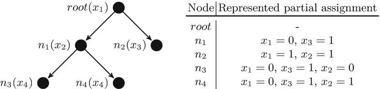
In this case, every node of the search tree represents a (partial) variable assignment and is marked with a variable that is unassigned in the node but becomes assigned in its children. The root node represents the empty assignment, i.e., an assignment where every variable is unassigned. 在这种情况下,搜索树的每个节点都表示一个(部分)变量分配,并用一个在节点中未分配但在其子节点中被分配的变量进行标记。根节点表示空赋值,即每个变量都未赋值的赋值。
Each non-root node n has a reference to its parent node (n.parent) and stores its parent’s variable assignment (n.assignment). We additionally define that each of this variable assignment must be an explicit assignment, i.e., an assignment that is not implied via unit propagation. 每个非根节点n都有对其父节点(n.parent)的引用,并存储其父节点的变量赋值(n.assignment)。此外,我们还定义每个变量赋值必须是显式赋值,即不通过单元传播隐含的赋值。
Then, each assignment represents the explicit assignment and all further assignments that follow via unit propagation. Using this definition, the assignments on the path from the root node to node n including all additional assignments that follow by unit propagation define the (partial) variable assignment of n. 然后,每个赋值表示显式赋值和通过单元传播遵循的所有进一步赋值。使用此定义,从根节点到节点n的路径上的赋值(包括单元传播之后的所有附加赋值)定义了n的(部分)变量赋值。 |
|
In Fig. 5.1, an exemplary search tree and the partial variable assignments that are represented by the search tree nodes for f = (¬x1 ∨ x2) ∧ (x1 ∨ x3) ∧ (x4 ∨ x5) are shown. For example, the variable assignment of node n3 contains the assignments x1 = 0 and x2 = 0, because they are the explicit assignments on the path from the root node to n3. Additionally it contains x3 = 1 as the assignment x1 = 0 and the clause (x1 ∨ x3) imply the assignment of x3 via unit propagation. Note that n1 and n2 have different variables in the example despite being children of the same node. This can happen as the assignment of x1 either implies the assignment of x2 or x3 and thus, dependent on the value of x1, either x2 or x3 does not need to be explicitly implied and cannot be the variable of a search tree node.
Fig. 5.1 Excerpt of a possible search tree and partial variable assignments of the search tree nodes for the formula f = (¬x1 ∨ x2) ∧ (x1 ∨ x3) ∧ (x4 ∨ x5). The variable of each node is notated in parenthesis behind the node name and we assume that the left child assigns the parent’s variable to zero, while the right child assigns it to one。
每个节点的变量在节点名后面的括号中表示,我们假设左子节点将父节点的变量赋值为零,而右子节点将其赋值为一. |
|
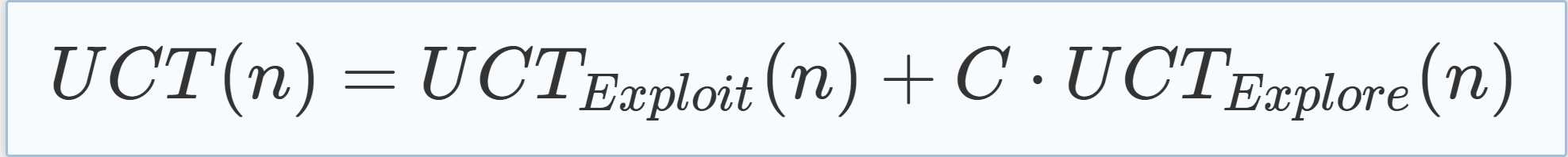
To be able to use the UCT formula, each node has an estimated value as well as a counter for the number of times the algorithm has traversed through it in the selection phase as explained below. Both of these properties, n.estimatedV alue and n.counter, are used to calculate the UCT value of a node n, where the UCT value of n consists of the exploration value as shown in Eq. (5.1) and the exploitation value as shown in Eq. (5.2). 为了能够使用UCT公式,每个节点都有一个估计值以及一个计数器,用于计算算法在选择阶段遍历它的次数,如下所述。 这两个属性n.estimatedV 值和n.counter用于计算节点n的UCT值,其中n的UCT值由等式(5.1)中所示的勘探值和等式(5.2)中所示的开采值组成. |
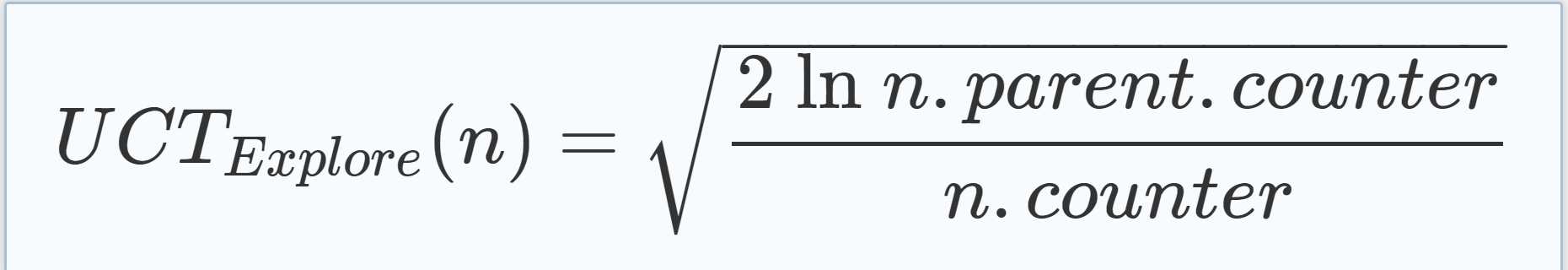 (5.1) (5.1) |
|
(5.2) |
|
n的UCT值可以通过将两个值相加来计算,如式(5.3)所示: |
|
(5.3) |
|
The factor C in Eq. (5.3) is the so-called exploration constant that can be used to weight the summands. Note that the algorithm never calculates the UCT value of the root node and thus n.parent.counter can safely be used as stated in Eq. (5.1). 式(5.3)中的系数C是所谓的勘探常数,可用于加权求和。注意,该算法从不计算根节点的UCT值,因此n.父计数器可安全使用,如式(5.1)所述。 |
|
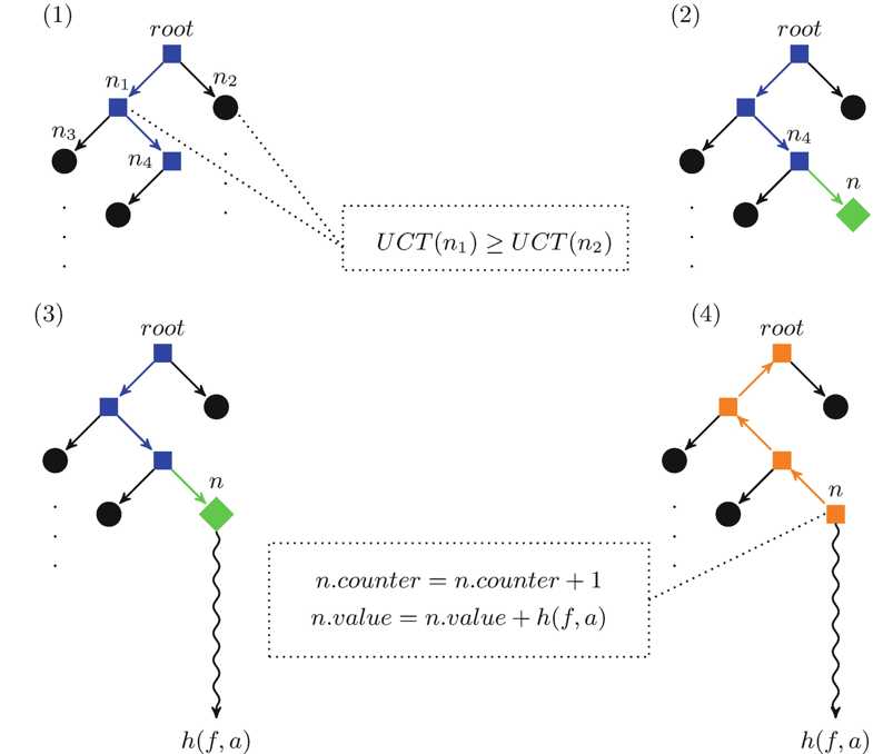
Given a CNF formula, the UCT based solver executes iterations until a satisfying assignment is found or the formula is proved to be unsatisfiable.给定一个CNF公式,基于UCT的解算器执行迭代,直到找到一个满意的赋值或证明该公式是不可满足的。 In each iteration, one node is added to the search tree, its value is estimated, and the values of the trees nodes are refreshed.在每次迭代中,会向搜索树中添加一个节点,估计其值,并刷新树节点的值。 During the iteration, an instance of the given formula is kept up to date by executing encountered assignments and—after each assignment—unit propagation on this formula.在迭代过程中,给定公式的实例通过执行遇到的赋值以及在该公式上的每个赋值单元传播之后保持最新。 The algorithm iterates through four phases—selection, expansion, simulation, and backpropagation—until a satisfying assignment is found or the root node is marked as conflicting and thus the formula is unsatisfiable. The four phases are explained in the following: 该算法通过四个阶段的选择、扩展、模拟和反向传播,直到找到一个满意的分配或根节点被标记为冲突(因此公式是不可满足的)。 这四个阶段的说明如下: |
In Fig. 5.2(1), the selection phase is illustrated. The square-shaped nodes are the nodes that are selected in the selection phase. We see that they form a path from the root to the fringe of the tree. In the example, n1 was selected instead of n2 because it has the higher UCT value. The selection phase stopped at node n4, because n4 only has one of the two possible children. |
|
Fig. 5.2 Illustration of one iteration through the four MCTS phases. (1) Selection phase: the graph is traversed starting from the root node along edges to nodes with higher UCT value until node n4 is reached (square-shaped nodes). (2) Expansion phase: a new child node representing an assignment for the variable of the parent node is added (diamond-shaped nodes). After the creation of the node, unit propagation is performed. (3) Simulation phase: starting from the partial assignment created by the new node, a simulation is started to compute the value h(f, a) that estimates the value of the new node. (4) Backpropagation phase: the estimation computed in the last step is propagated back through the nodes previously traversed to find the expansion point (square-shaped nodes). |
|
|
|
|
As already mentioned, the learning and usage of new clauses is a key aspect of modern SAT solvers. This section introduces the concept of Conflict-Driven Clause Learning and shows how it can be used in the MCTS-based algorithm.如前所述,学习和使用新的从句是现代SAT解译者的一个关键方面。本节介绍冲突驱动子句学习的概念,并说明如何将其用于基于MCTS的算法。 |
| Afterwards, we will analyze the behavior of the algorithm by visualizing the search trees that are produced by the MCTS-based CDCL solver. 然后,我们将通过可视化由基于MCTS的CDCL求解器生成的搜索树来分析算法的行为。 |
| The clause learning usually takes place whenever a conflict occurs and determines a new clause that formulates the reason for the conflict. The new clause is learned using an implication graph that is defined by the assigned variables and the clauses that implied assignments due to unit propagation and added to the overall formula. For a more detailed explanation on clause learning, see [10]. In the following, the integration of CDCL into an MCTS-based solver that was first presented in [14] is introduced. |
| This approach for an MCTS-based CDCL solver learns a new clause whenever a simulation leads to a conflict or a conflicting node is detected in the search tree and to add it to the formula when the algorithm starts a new iteration. The main aspect to consider is that at each node that is created during the expansion phase of the algorithm, a number of variables are already assigned to a value. While no node is created that has a variable assignment that directly causes a conflict, the learning of additional clauses can lead to the existence of nodes that have assignments which lead to a conflict in one of the learned clauses. As those nodes do not lead to a solution, they can be pruned from the search tree. Therefore we modify the algorithm to check the nodes that are traversed through during the selection phase for such conflicts. |
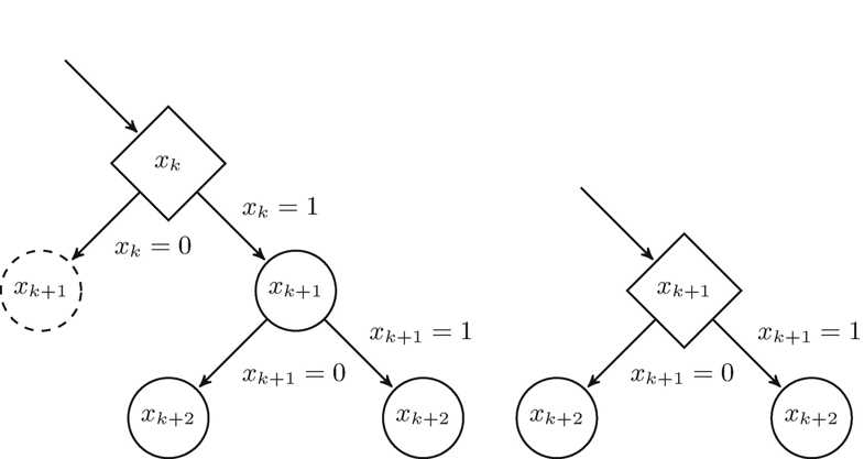
| The left part of Fig. 5.3 shows a situation where the algorithm is determining the successor of the diamond-shaped node formed during the selection phase and notices that assigning the current variable xk to 0 would lead to a conflict such that the dashed node is conflicting. |
|
Fig. 5.3 Encountering (left) and resolving (right) a conflicting node during the selection phase |
| The figure shows that the algorithm only has the choice to select the assignment xk = 1 because the alternative would lead into a conflict. At this point, there are two possible reasons for this conflict. First, the variable assignment could directly lead to the conflict and second, the unit propagation after the assignment could lead to the conflict. |
| If the variable assignment would directly lead into a conflict, it would mean that a clause C must exist which is unit in the variable assignment of the current node and has the unit literal xk. This is an important aspect as the algorithm was defined to execute unit propagation after each variable assignment, so after assigning the precursor variables of xk, the unit propagation must have already led to the assignment xk = 1. Because of that, not only the dashed node becomes unnecessary but also the diamond-shaped one as its variable must already have been assigned, so the algorithm can prune both nodes—including the child nodes of the conflicting node—and continue in the state shown in the right part of Fig. 5.3. |
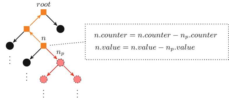
| To detect this case, the algorithm only has to check if the variable of the current node has already been assigned due to unit propagation. If, on the other hand, the unit propagation after the assignment xk = 0 leads to the conflict, the diamond-shaped node does not become redundant as its assignment was not already executed due to unit propagation in the previous nodes. In this case, the dashed node can still be pruned, but the diamond-shaped one needs to be retained. This case can be detected by checking whether a variable assignment led to a conflict during the selection phase. Note that if this second case occurs, a new conflict was found and thus a new clause is learned. Because this newly learned clause could lead to previous visited nodes becoming conflicting, we adjust the algorithm to directly execute the backpropagation phase and afterwards start a new iteration whenever this case occurs. The backpropagation phase is modified to take into account that parts of the search tree can never be reached again. Let v be a node that is removed from the search tree because it was detected to be conflicting. Another aspect to consider is that for each iteration i of the algorithm that traversed through v, the estimated value of i was backpropagated from v to the root node whereupon also the counter of all nodes on the path from v to the root was increased. Therefore iterations after the pruning of v would make decisions in the selection phase based on simulations in parts of the search space that can never be reached again. To prevent this, we modify the backpropagation phase to subtract the estimated value and counter of node v from the estimated value and counter of all nodes on the path from the root to v. |
|
Figure 5.4 illustrates the modification by showing that if a search tree node np—and consequently all of it successors, as highlighted by the dotted nodes in the figure—is pruned, the values of all nodes on the path from the direct predecessor of np to the root nodes are refreshed. The affected nodes are indicated by square-shaped nodes. The refreshment of the values is exemplary shown for node n. |
|
Fig. 5.4 Illustration of the modified backpropagation phase that occurs if a node np inside the search tree is pruned during the selection phase |
| Note that starting a new iteration from the root node of the tree instead of executing a backjump comes with an advantage of being able to choose the most promising point (according to the UCT formula) to continue the solving process. A backjump simply continues at the last node that is known to be conflict free. |
| To analyze the behavior of the algorithm, we implemented the MCTS-based CDCL Solver, used it to solve various benchmark problems, and were able to confirm that the addition of CDCL significantly improves the performance of the algorithm in comparison to the pure MCTS-based solver. As the detailed benchmark results can be found in [14], we will only exemplary illustrate the performance improvement by using visualizations of the search trees produced by the algorithm. The problems that were solved to create the search trees were taken from http://www.cs.ubc.ca/~hoos/SATLIB/benchm.html. |
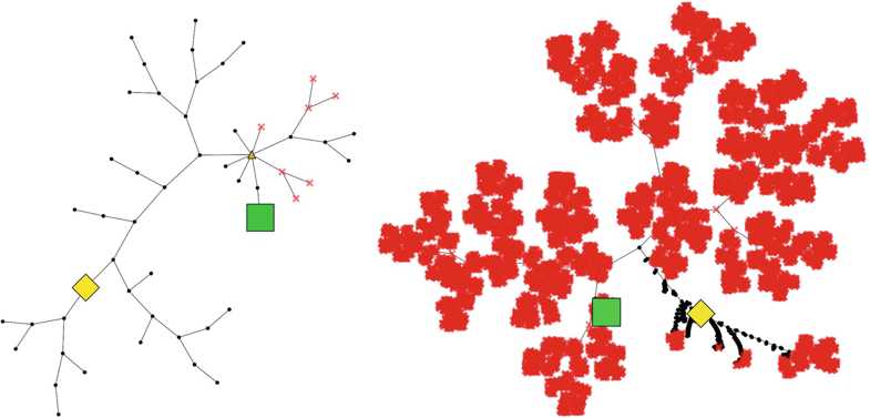
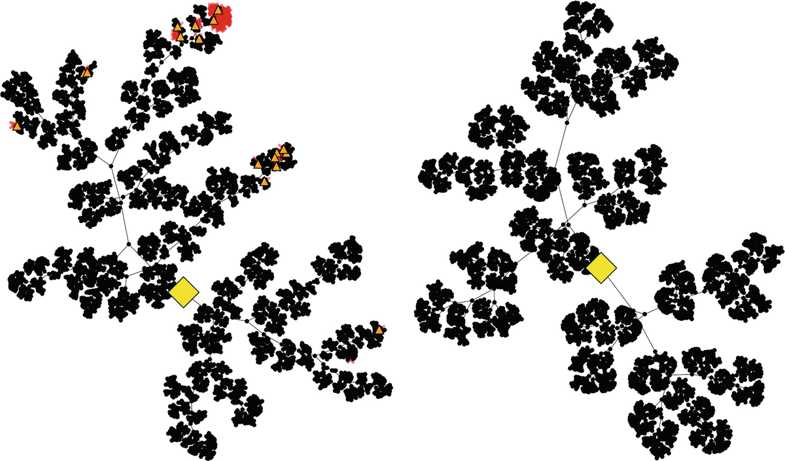
| The visualizations mark nodes that could be pruned as opaque crosses, if they were pruned because they were conflicting and as triangles, if they were found out to be redundant, i.e., if their assignment was already enforced by unit propagation on the learned clauses (see Sect. 5.3). Additionally the root node of the tree is highlighted as a diamond and the starting point of the simulation that eventually found a solution is highlighted as a square. The executed simulations are not shown in the visualization. |
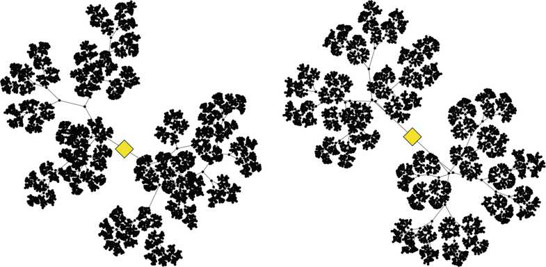
| Figure 5.5 illustrates the main benefits of CDCL by showing that the algorithm that actually used CDCL was able to create a much smaller search tree by pruning nodes near the root of the tree and exploiting unit propagation to find a solution near the root. The comparison of both trees indicates that two benefits of the addition of CDCL are the reduction of the memory needed to store the search tree and the running time to execute the simulations. This benefits are confirmed by the benchmark results in [14]. |
|
Fig. 5.5 Search trees produced by the MCTS-based solver with (left) and without clause learning on the graph coloring problem sw100-68 with 500 variables and 3100 clauses |
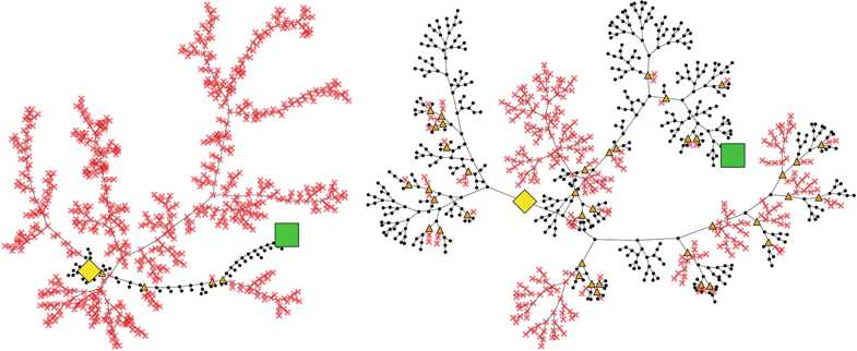
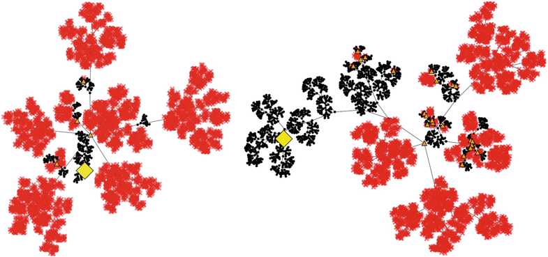
| To illustrate another benefit of MCTS, Fig. 5.6 compares the search trees of an algorithm with a low and high value for the exploration constant. The left search tree shows that the algorithm focused on expanding the search tree at the top of the picture and was able to prune whole branches before finding the solution. In contrast we see that the branches at the bottom of the picture are merely unexplored, because they were ignored due to a low estimated value. In contrast, the right tree is more equally explored in every direction. |
|
Fig. 5.6 Search trees produced by an algorithm with a small (left) and large exploration constant on the planning problem logistics.a with 828 variables and 6718 clauses |
| In this example, the variant with the small exploration constant worked better and was able to find a solution in less time and with a smaller search tree. One clearly sees that the used heuristics led the search into the correct direction and thus the exploitation in this direction turned out to be a good choice. In contrast the variant with a large exploration constant wasted time exploring other branches. While the usage of a low exploration constant turned out to be successful for this example, it highly relies on the usage of accurate heuristics and on accurate value estimations for the tree nodes. |
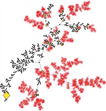
| Despite all these advantages, the MCTS-based CDCL solver was still not able to compete with state-of-the-art solvers and to solve hard instances. Nevertheless, when visualizing the search trees that were produced on harder instances (see Fig. 5.7, for example), the trees still showed the same characteristics as the ones we analyzed before. In particular, the algorithm was often still able to prune the search tree near to its root, because of the learned clauses. |
|
Fig. 5.7 Search tree produced by the MCTS-based CDCL solver in the first 10 s of solving a pigeon hole instance with 14 holes. See, e.g. [5] for a definition of the pigeon hole problem |
| As such clauses are valuable because they reduce the search space by a large factor, the question arises whether one can take advantage of the algorithm’s ability to learn them. The next sections of the chapter will discuss how the MCTS-based CDCL solver can be used to actively search for “good” clauses and how to take advantage of them. |
| While the performance improvement was the main motivation to use CDCL in combination with MCTS, the usage of CDCL also gives access to more information about the problem that is to be solved. Obviously, the learned clauses themselves are additional knowledge about the problem, but there is also the possibility to collect statistics about the clause learning process. This section introduces MCTS specific heuristics that exploit the described information. |
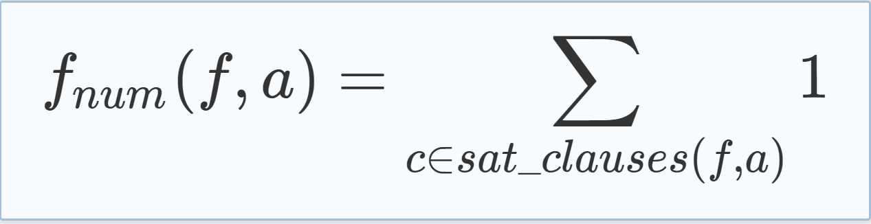
| In Sect. 5.2, the scoring mechanism of the MCTS-based SAT solver was introduced and defined to use the number of satisfied clauses as a measurement for the quality of a simulation. This is very intuitive as the goal of the solver is to satisfy all clauses and thus the maximization of the number of satisfied clauses—like in the MaxSAT problem—is the consequent approach. While this measurement was successfully used in the MCTS-based SAT solver with and without clause learning, this section presents alternative measurements to adapt to the addition of CDCL to the plain algorithm. This gives access to more information during the course of the algorithm that can be exploited in the scoring heuristic. |
| One common approach when designing SAT solving heuristics is to accredit more importance to clauses and variables that have a high impact on the clause learning procedure. For example, the learning rate based heuristic [8] uses such a measurement to order the variables. |
| There are different ways to define scoring heuristics that follow this approach, where the easiest one is the initially introduced heuristic that just uses the number of satisfied clauses as a measurement (see Eq. (5.4), where sat_clauses(f, a) is the set of satisfied clauses in formula f for the variable assignment a). When this heuristic is used in the context of the MCTS-based CDCL algorithm, the number of clauses raises through the course of its execution and thus the fulfillment of learned clauses gains extra importance by enabling higher scores. |
|
(5.4) |
|
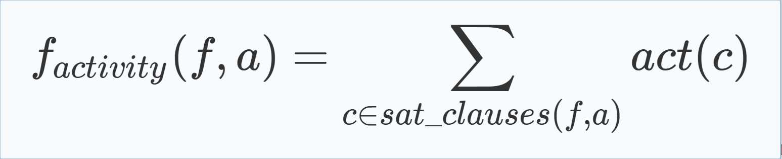
To explain a second scoring heuristic that follows the described approach we define the activity act(c) of a clause c as the number of times c occurred during the resolution process of the clause learning procedure. Equation (5.5) uses this measurement to benefit the satisfying of clauses with high activity values. We also tried a similar scoring heuristic that is inspired by the VSIDS variable order heuristic which benefits variables that occur in newly learned clauses and uses the age of clauses, i.e., the number of MCTS iterations that occurred since the clauses were added, to benefit the satisfying of new clauses. This heuristic behaved similarly and thus is not further considered. |
|
(5.5) |
| Another approach is to not directly optimize the satisfying of as many clauses as possible but to optimize the collection of useful information. As already concluded in the analysis of the search trees, a great benefit of the MCTS-based CDCL solver may be the ability to learn valuable clauses. We now introduce different heuristics that aim on learning clauses that fulfill different criteria and reward the learning of “good” clauses. One simple and commonly used criteria for the quality of learned clauses is their length, which leads to the scoring heuristic as defined in Eq. (5.6), where length(c) is the number of literals in the newly learned clause c. |
|
(5.6) |
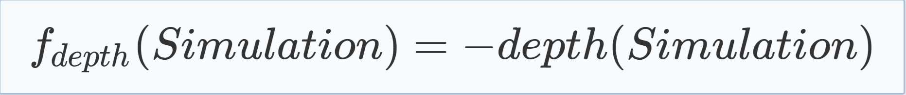
| Another criterion to measure the quality of learned clauses is to benefit the learning of clauses that enable the algorithm to cut the search space near to its root. To do so, we define fdepth in Eq. (5.7)—where depth(s) is the number of decisions, i.e., variable assignments that were not caused by unit propagation, that were executed in a simulation s—that rewards simulations which lead to a conflict after a low number of decisions and therefore learn clauses that prune the search tree near to its root. |
|
(5.7) |
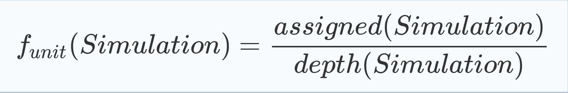
| A last scoring heuristic aims to reward simulations that enforce many variable assignments due to unit propagation. As formulated in Eq. (5.8), where assigned(s) is the number of variables that were assigned in simulation s, the heuristic gives those simulations a high value that executed a high proportion of their assignments due to unit propagation. |
|
(5.8) |
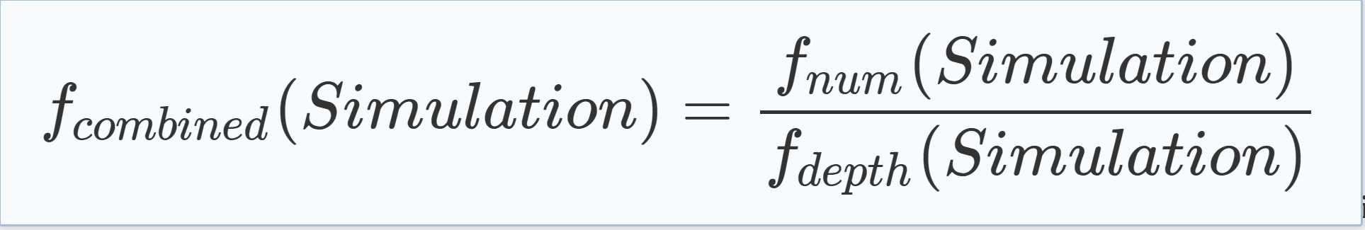
| Of course, the different heuristics can be combined to follow both approaches or benefit different criteria. For example, one could reward the occurrence of early conflicts while satisfying as many clauses as possible (see Eq. (5.9)). |
|
(5.9) |
| In Sect. 5.6 we will see that the different heuristics succeed in optimizing their respective criteria. |
| n Sect. 5.2 the simulations of the MCTS-based CDCL solver were defined to assign the variables of the formula uniformly at random. While this is an approach that can be used to solve SAT and is quite standard when using MCTS, it is also common to use domain specific knowledge—if it is available—to weight the probabilities in the simulation phase [1]. This section focuses on using knowledge that can be extracted from the given SAT formula as well as from the learned clauses to weight the probabilities. |
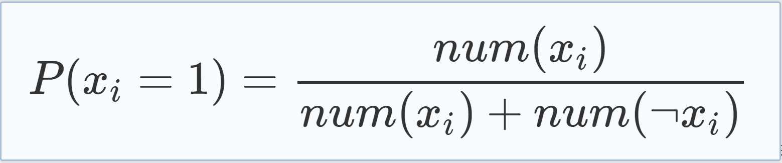
| In backtracking-based SAT solvers, the decision to which value to assign the variables is made using the Phase Selection Heuristic, where one approach is to assign a variable xi to 1 if the literal xi occurs more often in the formula than ¬xi and vice versa. We adapted this approach and used probabilities according to Eq. (5.10) during the simulation phase, where num(xi) is the number of occurrences of literal xi in the formula and P(xi = 1) is the probability of assigning variable xi to 1. |
|
(5.10) |
| Note that the number of occurrences of a literal in the formula changes during the course of the algorithm because of the newly added clauses. We experimented with different probabilities when solving benchmark problems, but were not able to reach clear results, meaning that for some problems the probabilities according to Eq. (5.10) performed better and for others the uniform random assignment outperformed the competitor. The results of this experiments can be found in [14]. |
| Because we were not able to obtain clear results on the benefits of using non-uniform probability heuristics, all experiments in Sect. 5.6 used the uniform random probability heuristic. |
| Similar to Sect. 5.3.2 we now will analyze the impact of the different heuristics by using visualizations of search trees that were produced using the heuristics. We therefore used the MCTS-based CDCL solver with different scoring heuristics to again solve a pigeon hole instance with 14 holes and in the following will use the produced search trees to exemplary analyze the impact of the heuristics. Later, in the experiments section, we will quantify the results of this exemplary analysis with more data. |
| As a starting point for the analysis, we will look at the search trees that were produced using the initially introduced scoring heuristic, i.e., the number of satisfied clauses after a simulation (fnum). Figure 5.8 shows the search trees produced 30 s into the solving with an exploration constant of 0.1 and 0.3. We again see that in both cases the search tree is asymmetric, but the variant with the higher exploration constant more intensely explored both branches of the root and the variant with the lower exploration constant was able to exploit its greedy nature to create and prune more nodes in the branch left of the root. |
|
Fig. 5.8 Search trees produced by the MCTS-based CDCL solver using the fnum scoring heuristic in the first 30 s of solving a pigeon hole instance with 14 holes using an exploration constant of 0.1 (left) and 0.3 (right) |
| In comparison, Fig. 5.9 shows the search trees of the same situation when the fdepth heuristic is used instead. We can observe that the share of pruned nodes is higher for both exploration constants than in the search trees that were produced using the fnum heuristic. This is exactly how the search trees should look like by design of the heuristic. As fdepth was designed to encourage early conflicts, it also encourages the pruning of nodes near the root, which explains the higher share of pruned nodes. A second aspect we can observe when comparing the search trees with an exploration constant of 0.3 is that the search tree that was produced using the fnum heuristic is “more symmetric” than the one that was produced using fdepth, meaning that the less explored branch of the root contains more nodes and thus the tree is more balanced. This means that the usage of heuristic fdepth led to clearer results on where to expand the search tree and thus one branch of the root node was more intensely exploited. |
|
Fig. 5.9 Search trees produced by the MCTS-based CDCL solver using the fdepth scoring heuristic in the first 30 s of solving a pigeon hole instance with 14 holes using an exploration constant of 0.1 (left) and 0.3 (right) |
| Therefore one could argue that the heuristic fdepth works better on this example, because the main goal of the algorithm is to be able to find and exploit areas of the search space where the heuristic leads to high scores. A more unbalanced tree means that the algorithm was more successful to do just that. |
| To further elaborate on this thought, we take a look at the search trees produced in the same situation while using the factivity heuristic as illustrated in Fig. 5.10. We can observe that the search trees produced for both exploration constants explored both branches of the root fairly equally and also led to quite balanced sub trees. Thus, the algorithm was not able to find areas of the search space such that the factivity heuristic reached high enough results to exploit. We can conclude that, by using the factivity heuristic, we do not gain any information about the problem as the results seem to be similar in all explored areas of the search space and the search tree is built more or less in a breadth-first search fashion. Therefore, the factivity heuristic probably is not a good choice for at least this example. |
|
Fig. 5.10 Search trees produced by the MCTS-based CDCL solver using the factivity scoring heuristic in the first 30 s of solving a pigeon hole instance with 14 holes using an exploration constant of 0.1 (left) and 0.3 (right) |
| To sum up the analysis, recap that we observed that the fdepth heuristic reached its design goal by successfully pruning more nodes near to the root node than the other heuristics. In the experiments section we will quantify this observation and investigate whether the other heuristics reach their design goals as well. We also observed that the heuristics differ in their ability to create asymmetric search trees and argued that this ability is an indicator if a heuristic can be successfully used for a specific problem. In the experiments section we will collect statistics on the symmetry of the search trees and quantify which heuristics succeed to create asymmetric trees for different problems. |
| In the previous sections we designed heuristics that enable an MCTS-based CDCL solver to actively search for “good” clauses. However, the current implementation of the algorithm cannot compete with established solvers. Therefore this section will focus on how to combine the MCTS-based approach with different solvers and thereby take advantage of the clauses learned by an MCTS-based algorithm that uses the previously introduced heuristics. As stated in the previous section, it is possible to configure the algorithm to optimize different SAT related aspects like the usage of unit propagation, the learning of short clauses, and the cutting of the search space near its root. All of these aspects are strongly related to the learned clauses. This leads to the assumption that different solvers can benefit from importing those clauses. |
| Our approach is to generate such clauses by running a portfolio of instances of the algorithm as a preprocessor for another solver. The MCTS-based solver instances of the portfolio are configured to encourage the pruning of the search tree, the learning of short clauses, and the usage of unit propagation by using the corresponding scoring heuristics that were introduced in Sect. 5.4. For a given SAT instance, the portfolio is run for a fixed time to learn clauses that benefit the mentioned aspects. After that, a backtracking-based solver is started on the given problem—including the previously learned clauses. The hypothesis is that these clauses improve the performance of the second solver, as they were learned to encourage the mentioned SAT related aspects. If the preprocessor was able to actually solve the given problem, the second solver is not started. |
| For the experiments described in Sect. 5.6, four instances of the MCTS-based CDCL solver are used to preprocess a backtracking-based CDCL solver. The instances were configured to use fdepth, funit, flength, respectively, fnum as scoring heuristics. The selection of this four heuristics will be explained in Sect. 5.6. As the experiments will show, the preprocessing was able to improve the performance of the backtracking-based algorithm on several benchmark problems. |
| In this chapter we analyzed the behavior of a Monte Carlo Tree Search-based Conflict-Driven Clause Learning SAT solver and showed that the usage of CDCL is beneficial for the SAT solving process. The improvement is achieved by pruning the search tree and directing the simulations in better directions via unit propagation on the learned clauses. |
| The visualization of the search trees indicates the importance of an accurate value estimation of the tree nodes as it enables the algorithm to ignore large parts of the search space. Additionally they illustrate the ability of the algorithm to learn valuable clauses. |
| To further take advantage of that ability, different scoring heuristics were introduced that can be used to actively search for valuable clauses. Our experiments showed that it is indeed possible to use those heuristics to configure the algorithm to optimize different SAT related aspects—like the learning of short clauses or the early occurrence of conflicts. |
| This fact was exploited by preprocessing SAT instances before handing them to other solvers. While a lot of open questions—like the duration of the preprocessing or which clauses to import—exist, the experiments indicate that the preprocessing can be very benefiting and improve the performance of established SAT solvers. As this result also indicates that other solvers can benefit from importing the clauses learned by our solver, we will investigate whether using the MCTS-based CDCL solver in a portfolio approach can be beneficial. This could be done either using the MCTS-based solver exclusively or by integrating it in a more diverse portfolio employing a range of different solvers. In its current development stage, our solver is not capable of competing with established SAT solvers as a stand-alone solver. Therefore we additionally will pursue the obvious next step of improving the solver by means of software engineering. |
决策变元选择_决策分支策略——文献学习Improving SAT Solving Using Monte Carlo Tree Search-Based Clause Learning
标签:logistic rman over 基础 loading lov backtrac 经典 reduce
原文地址:https://www.cnblogs.com/yuweng1689/p/13198505.html