机器学习sklearn（十一）： 数据处理（六）非线性转换

标签：lob   fun   instance   正数   res   john   apply   pass   gen   

有两种类型的转换是可用的:分位数转换和幂函数转换。分位数和幂变换都基于特征的单调变换，从而保持了每个特征值的秩。

通过执行秩变换，分位数变换平滑了异常分布，并且比缩放方法受异常值的影响更小。但是它的确使特征间及特征内的关联和距离失真了。

幂变换则是一组参数变换，其目的是将数据从任意分布映射到接近高斯分布的位置。

1 映射到均匀分布

QuantileTransformer 类以及 quantile_transform 函数提供了一个基于分位数函数的无参数转换，将数据映射到了零到一的均匀分布上:

>>> from sklearn.datasets import load_iris
>>> from sklearn.model_selection import train_test_split
>>> iris = load_iris()
>>> X, y = iris.data, iris.target
>>> X_train, X_test, y_train, y_test = train_test_split(X, y, random_state=0)
>>> quantile_transformer = preprocessing.QuantileTransformer(random_state=0)
>>> X_train_trans = quantile_transformer.fit_transform(X_train)
>>> X_test_trans = quantile_transformer.transform(X_test)
>>> np.percentile(X_train[:, 0], [0, 25, 50, 75, 100])
array([ 4.3,  5.1,  5.8,  6.5,  7.9])

这个特征是萼片的厘米单位的长度。一旦应用分位数转换，这些元素就接近于之前定义的百分位数:

>>> np.percentile(X_train_trans[:, 0], [0, 25, 50, 75, 100])
...
array([ 0.00... ,  0.24...,  0.49...,  0.73...,  0.99... ])

这可以在具有类似形式的独立测试集上确认:

>>> np.percentile(X_test[:, 0], [0, 25, 50, 75, 100])
...
array([ 4.4  ,  5.125,  5.75 ,  6.175,  7.3  ])
>>> np.percentile(X_test_trans[:, 0], [0, 25, 50, 75, 100])
...
array([ 0.01...,  0.25...,  0.46...,  0.60... ,  0.94...])

2 映射到高斯分布

在许多建模场景中，需要数据集中的特征的正态化。幂变换是一类参数化的单调变换， 其目的是将数据从任何分布映射到尽可能接近高斯分布，以便稳定方差和最小化偏斜。

类 PowerTransformer 目前提供两个这样的幂变换,Yeo-Johnson transform 和 the Box-Cox transform。

Yeo-Johnson transform:

Box-Cox transform:

 Box-Cox只能应用于严格的正数据。在这两种方法中，变换都是参数化的，通过极大似然估计来确定。下面是一个使用Box-Cox将样本从对数正态分布映射到正态分布的示例:

>>> pt = preprocessing.PowerTransformer(method=‘box-cox‘, standardize=False)
>>> X_lognormal = np.random.RandomState(616).lognormal(size=(3, 3))
>>> X_lognormal                                         
array([[1.28..., 1.18..., 0.84...],
       [0.94..., 1.60..., 0.38...],
       [1.35..., 0.21..., 1.09...]])
>>> pt.fit_transform(X_lognormal)                   
array([[ 0.49...,  0.17..., -0.15...],
       [-0.05...,  0.58..., -0.57...],
       [ 0.69..., -0.84...,  0.10...]])

上述示例设置了参数standardize的选项为 False 。 但是，默认情况下，类PowerTransformer将会应用zero-mean,unit-variance normalization到变换出的输出上。

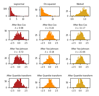
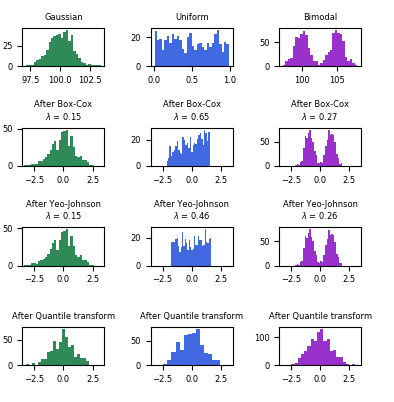
下面的示例中 将 Box-Cox 和 Yeo-Johnson 应用到各种不同的概率分布上。 请注意 当把这些方法用到某个分布上的时候， 幂变换得到的分布非常像高斯分布。但是对其他的一些分布，结果却不太有效。这更加强调了在幂变换前后对数据进行可视化的重要性。

 我们也可以 使用类 QuantileTransformer (通过设置 output_distribution=‘normal‘)把数据变换成一个正态分布。下面是将其应用到iris dataset上的结果:

>>> quantile_transformer = preprocessing.QuantileTransformer(
...     output_distribution=‘normal‘, random_state=0)
>>> X_trans = quantile_transformer.fit_transform(X)
>>> quantile_transformer.quantiles_
array([[4.3, 2. , 1. , 0.1],
       [4.4, 2.2, 1.1, 0.1],
       [4.4, 2.2, 1.2, 0.1],
       ...,
       [7.7, 4.1, 6.7, 2.5],
       [7.7, 4.2, 6.7, 2.5],
       [7.9, 4.4, 6.9, 2.5]])

因此，输入的中值变成了输出的均值，以0为中心。正态输出被裁剪以便输入的最大最小值(分别对应于1e-7和1-1e-7)不会在变换之下变成无穷。

API 

class sklearn.preprocessing.QuantileTransformer(*, n_quantiles=1000, output_distribution=‘uniform‘, ignore_implicit_zeros=False, subsample=100000, random_state=None, copy=True)

Transform features using quantiles information.

This method transforms the features to follow a uniform or a normal distribution. Therefore, for a given feature, this transformation tends to spread out the most frequent values. It also reduces the impact of (marginal) outliers: this is therefore a robust preprocessing scheme.

The transformation is applied on each feature independently. First an estimate of the cumulative distribution function of a feature is used to map the original values to a uniform distribution. The obtained values are then mapped to the desired output distribution using the associated quantile function. Features values of new/unseen data that fall below or above the fitted range will be mapped to the bounds of the output distribution. Note that this transform is non-linear. It may distort linear correlations between variables measured at the same scale but renders variables measured at different scales more directly comparable.

Read more in the User Guide.

Parameters

n_quantilesint, default=1000 or n_samples

Number of quantiles to be computed. It corresponds to the number of landmarks used to discretize the cumulative distribution function. If n_quantiles is larger than the number of samples, n_quantiles is set to the number of samples as a larger number of quantiles does not give a better approximation of the cumulative distribution function estimator.

output_distribution{‘uniform’, ‘normal’}, default=’uniform’

Marginal distribution for the transformed data. The choices are ‘uniform’ (default) or ‘normal’.

ignore_implicit_zerosbool, default=False

Only applies to sparse matrices. If True, the sparse entries of the matrix are discarded to compute the quantile statistics. If False, these entries are treated as zeros.

subsampleint, default=1e5

Maximum number of samples used to estimate the quantiles for computational efficiency. Note that the subsampling procedure may differ for value-identical sparse and dense matrices.

random_stateint, RandomState instance or None, default=None

Determines random number generation for subsampling and smoothing noise. Please see subsample for more details. Pass an int for reproducible results across multiple function calls. See Glossary

copybool, default=True

Set to False to perform inplace transformation and avoid a copy (if the input is already a numpy array).

Attributes

n_quantiles_int

The actual number of quantiles used to discretize the cumulative distribution function.

quantiles_ndarray of shape (n_quantiles, n_features)

The values corresponding the quantiles of reference.

references_ndarray of shape (n_quantiles, )

Quantiles of references.

Examples

>>> import numpy as np
>>> from sklearn.preprocessing import QuantileTransformer
>>> rng = np.random.RandomState(0)
>>> X = np.sort(rng.normal(loc=0.5, scale=0.25, size=(25, 1)), axis=0)
>>> qt = QuantileTransformer(n_quantiles=10, random_state=0)
>>> qt.fit_transform(X)
array([...])

API

class sklearn.preprocessing.PowerTransformer(method=‘yeo-johnson‘, *, standardize=True, copy=True)

Apply a power transform featurewise to make data more Gaussian-like.

Power transforms are a family of parametric, monotonic transformations that are applied to make data more Gaussian-like. This is useful for modeling issues related to heteroscedasticity (non-constant variance), or other situations where normality is desired.

Currently, PowerTransformer supports the Box-Cox transform and the Yeo-Johnson transform. The optimal parameter for stabilizing variance and minimizing skewness is estimated through maximum likelihood.

Box-Cox requires input data to be strictly positive, while Yeo-Johnson supports both positive or negative data.

By default, zero-mean, unit-variance normalization is applied to the transformed data.

Read more in the User Guide.

Parameters

method{‘yeo-johnson’, ‘box-cox’}, default=’yeo-johnson’

The power transform method. Available methods are:

• ‘yeo-johnson’ [1], works with positive and negative values

• ‘box-cox’ [2], only works with strictly positive values

standardizebool, default=True

Set to True to apply zero-mean, unit-variance normalization to the transformed output.

copybool, default=True

Set to False to perform inplace computation during transformation.

Attributes

lambdas_ndarray of float of shape (n_features,)

The parameters of the power transformation for the selected features.

Examples

>>> import numpy as np
>>> from sklearn.preprocessing import PowerTransformer
>>> pt = PowerTransformer()
>>> data = [[1, 2], [3, 2], [4, 5]]
>>> print(pt.fit(data))
PowerTransformer()
>>> print(pt.lambdas_)
[ 1.386... -3.100...]
>>> print(pt.transform(data))
[[-1.316... -0.707...]
 [ 0.209... -0.707...]
 [ 1.106...  1.414...]]

机器学习sklearn（十一）： 数据处理（六）非线性转换

标签：lob   fun   instance   正数   res   john   apply   pass   gen   

原文地址：https://www.cnblogs.com/qiu-hua/p/14903554.html