【树叶分类】基于matlab GUI BP神经网络植物叶片识别分类【含Matlab源码 916期】

标签：ring   偏差   形式   --   max   前馈网络   object   差值   要求   

一、简介

1 概述
BP（Back Propagation）神经网络是1986年由Rumelhart和McCelland为首的科研小组提出，参见他们发表在Nature上的论文 Learning representations by back-propagating errors 。

BP神经网络是一种按误差逆传播算法训练的多层前馈网络，是目前应用最广泛的神经网络模型之一。BP网络能学习和存贮大量的 输入-输出模式映射关系，而无需事前揭示描述这种映射关系的数学方程。它的学习规则是使用最速下降法，通过反向传播来不断 调整网络的权值和阈值，使网络的误差平方和最小。

2 BP算法的基本思想
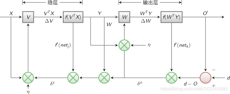
上一次我们说到，多层感知器在如何获取隐层的权值的问题上遇到了瓶颈。既然我们无法直接得到隐层的权值，能否先通过输出层得到输出结果和期望输出的误差来间接调整隐层的权值呢？BP算法就是采用这样的思想设计出来的算法，它的基本思想是,学习过程由信号的正向传播与误差的反向传播两个过程组成。
正向传播时，输入样本从输入层传入,经各隐层逐层处理后,传向输出层。若输出层的实际输出与期望的输出(教师信号)不符,则转入误差的反向传播阶段。
反向传播时，将输出以某种形式通过隐层向输入层逐层反传,并将误差分摊给各层的所有单元,从而获得各层单元的误差信号,此误差信号即作为修正各单元权值的依据。
这两个过程的具体流程会在后文介绍。

BP算法的信号流向图如下图所示

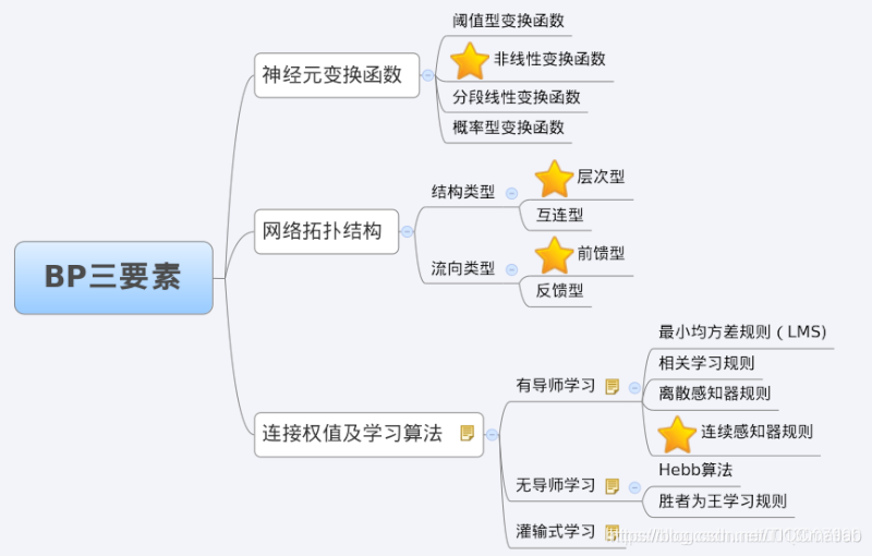
3 BP网络特性分析——BP三要素
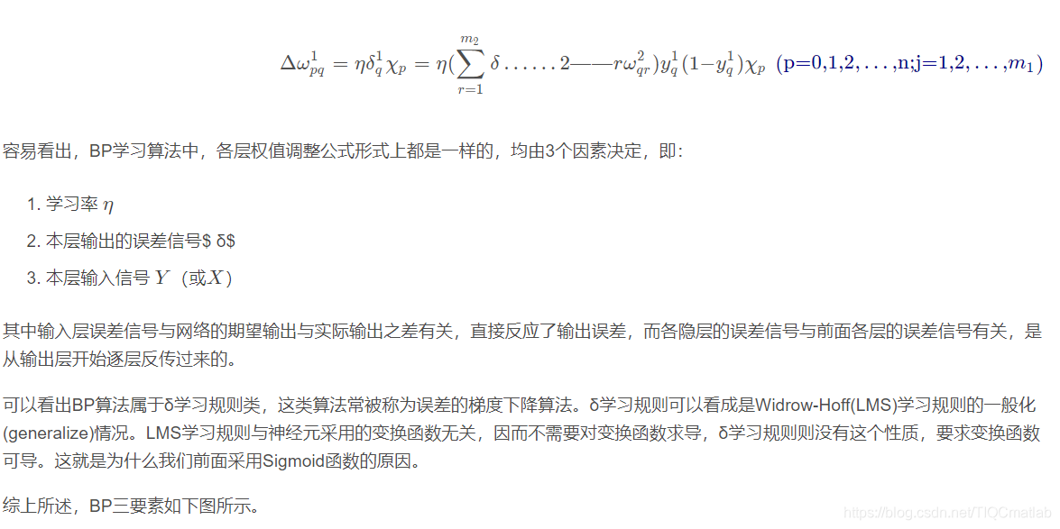
我们分析一个ANN时，通常都是从它的三要素入手，即
1)网络拓扑结构；
2)传递函数；
3)学习算法。

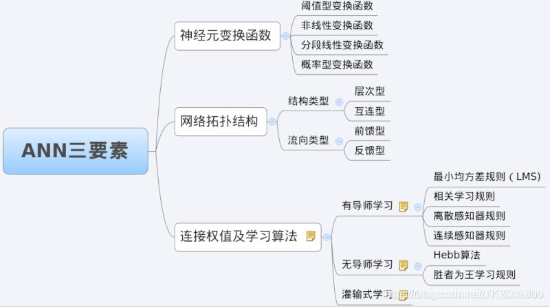
每一个要素的特性加起来就决定了这个ANN的功能特性。所以，我们也从这三要素入手对BP网络的研究。
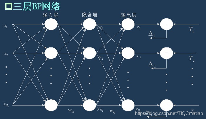
3.1 BP网络的拓扑结构
上一次已经说了，BP网络实际上就是多层感知器，因此它的拓扑结构和多层感知器的拓扑结构相同。由于单隐层（三层）感知器已经能够解决简单的非线性问题，因此应用最为普遍。三层感知器的拓扑结构如下图所示。
一个最简单的三层BP：

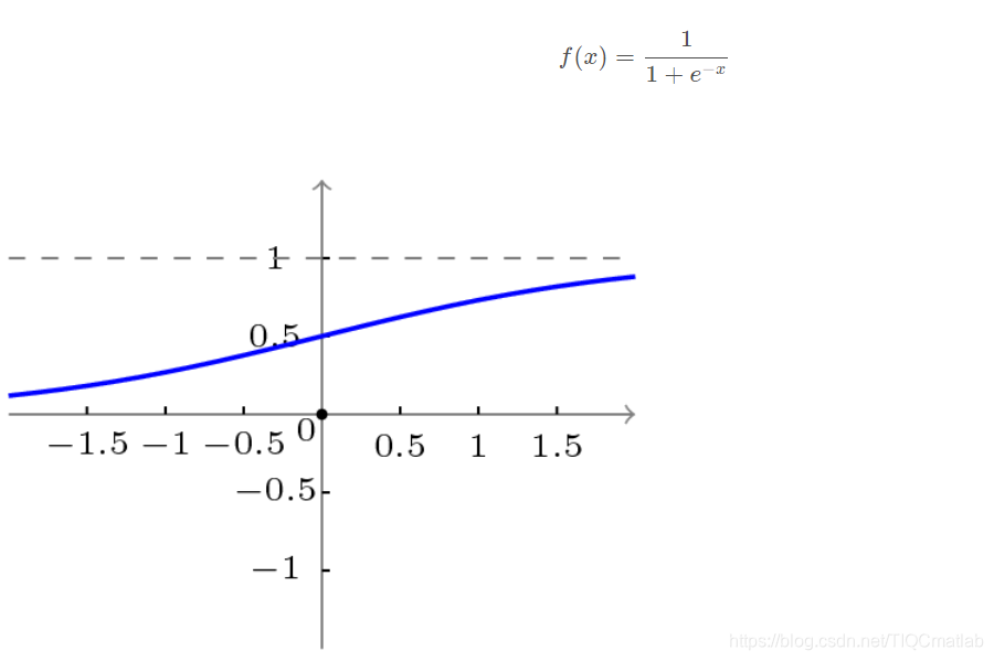
3.2 BP网络的传递函数
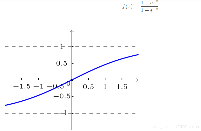
BP网络采用的传递函数是非线性变换函数——Sigmoid函数（又称S函数）。其特点是函数本身及其导数都是连续的，因而在处理上十分方便。为什么要选择这个函数，等下在介绍BP网络的学习算法的时候会进行进一步的介绍。
单极性S型函数曲线如下图所示。

双极性S型函数曲线如下图所示。

3.3 BP网络的学习算法
BP网络的学习算法就是BP算法，又叫 δ 算法（在ANN的学习过程中我们会发现不少具有多个名称的术语）， 以三层感知器为例，当网络输出与期望输出不等时，存在输出误差 E ，定义如下




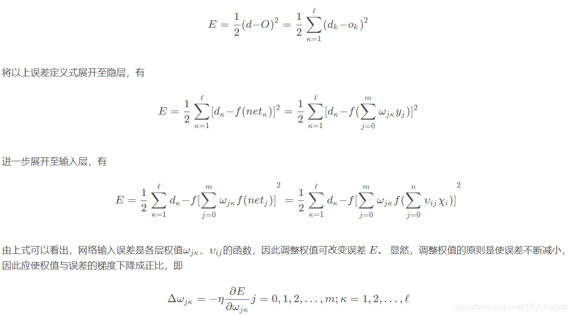
下面我们会介绍BP网络的学习训练的具体过程。

4 BP网络的训练分解
训练一个BP神经网络，实际上就是调整网络的权重和偏置这两个参数，BP神经网络的训练过程分两部分：

前向传输，逐层波浪式的传递输出值；
逆向反馈，反向逐层调整权重和偏置；
我们先来看前向传输。
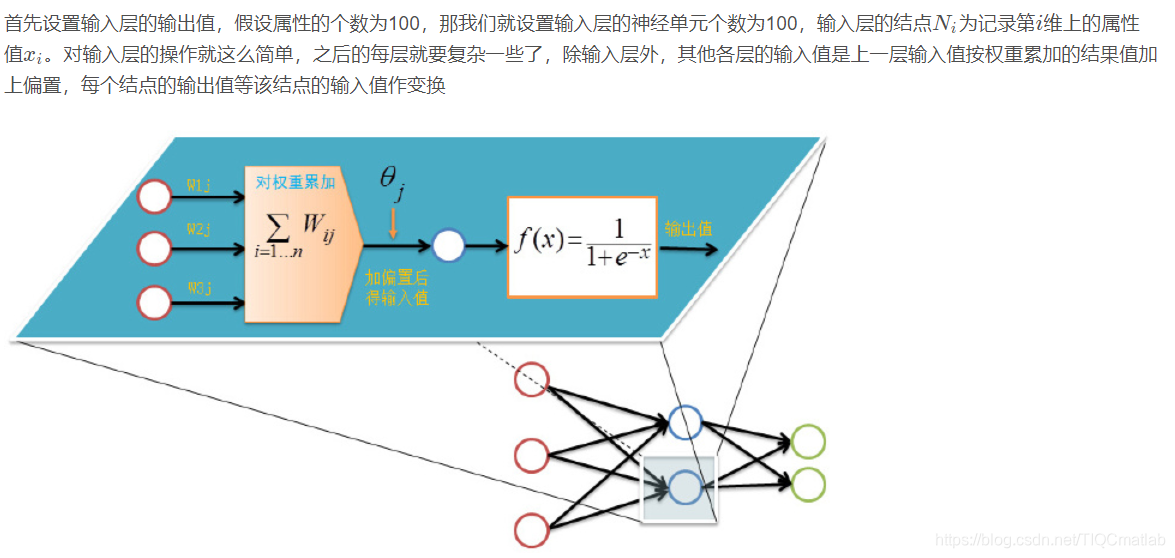
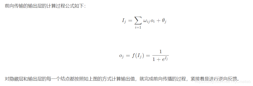
前向传输（Feed-Forward前向反馈）
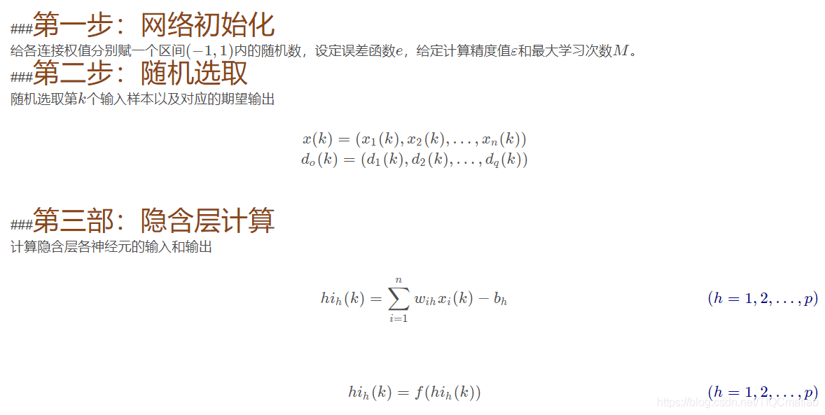
在训练网络之前，我们需要随机初始化权重和偏置，对每一个权重取[ ? 1 , 1 ] [-1,1][?1,1]的一个随机实数，每一个偏置取[ 0 , 1 ] [0,1][0,1]的一个随机实数，之后就开始进行前向传输。

神经网络的训练是由多趟迭代完成的，每一趟迭代都使用训练集的所有记录，而每一次训练网络只使用一条记录，抽象的描述如下：

while 终止条件未满足：
    for record:dataset:
        trainModel(record)

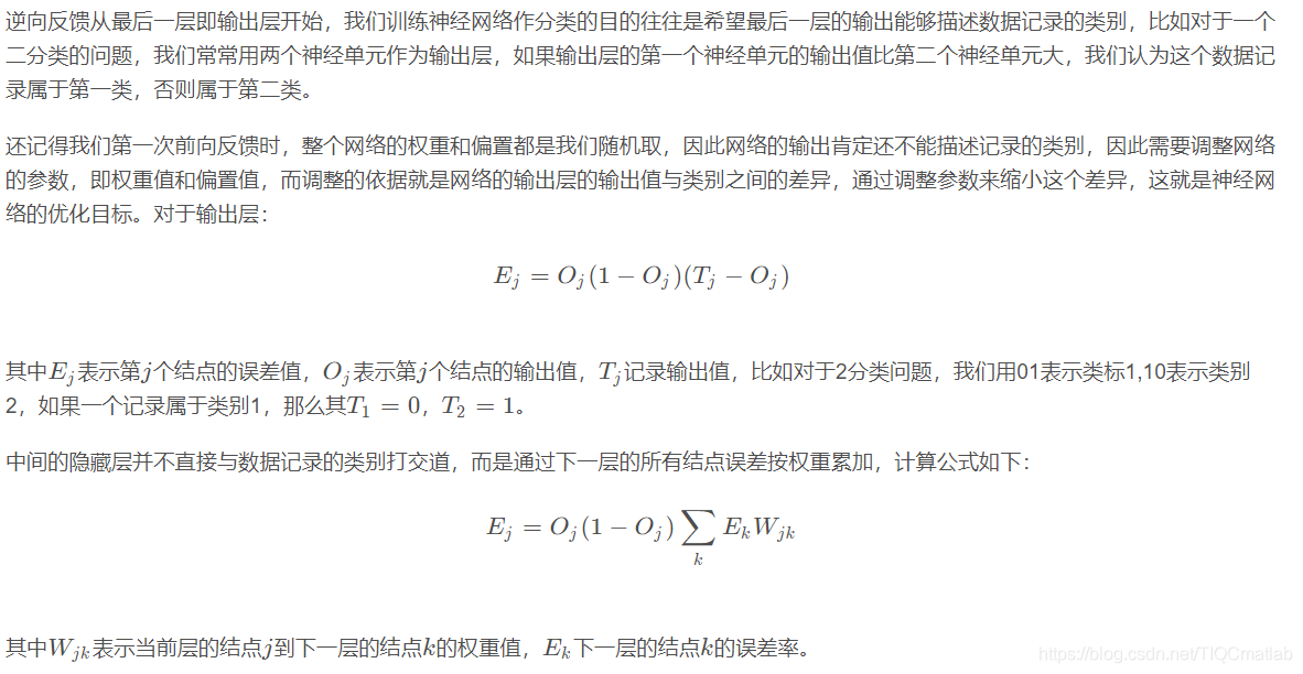
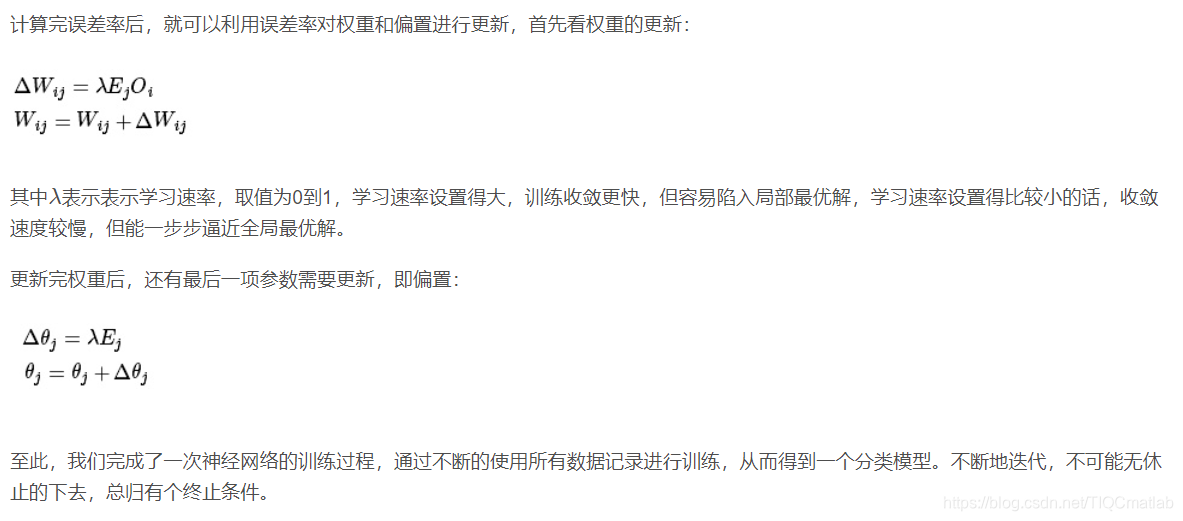
4.1 逆向反馈（Backpropagation）


4.2 训练终止条件
每一轮训练都使用数据集的所有记录，但什么时候停止，停止条件有下面两种：
设置最大迭代次数，比如使用数据集迭代100次后停止训练
计算训练集在网络上的预测准确率，达到一定门限值后停止训练

5 BP网络运行的具体流程
5.1 网络结构
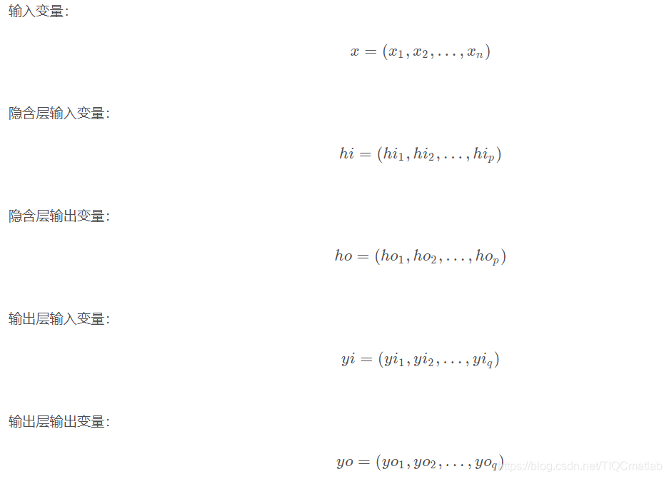
输入层有n nn个神经元，隐含层有p pp个神经元，输出层有q qq个神经元。
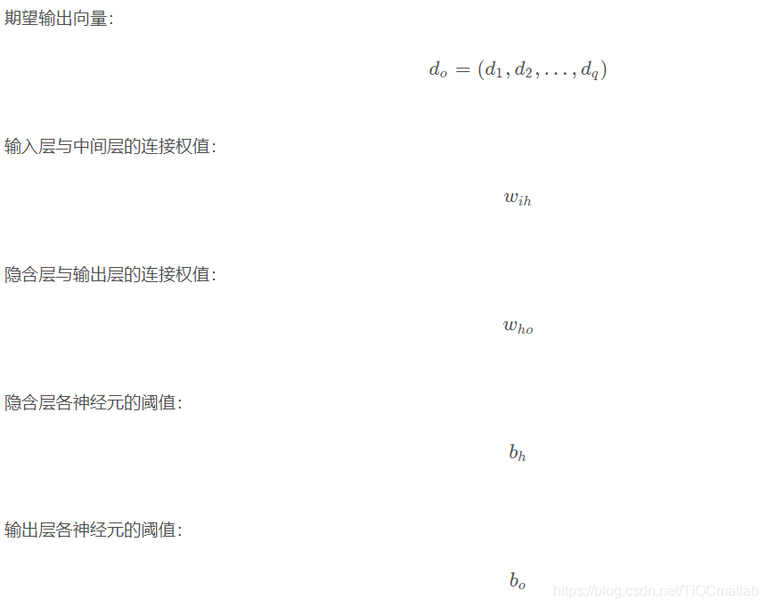
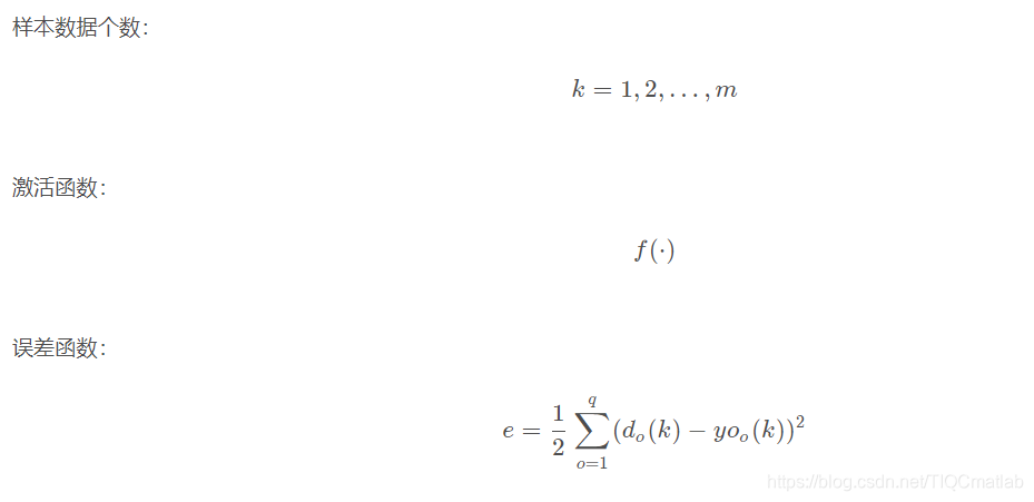
5.2 变量定义








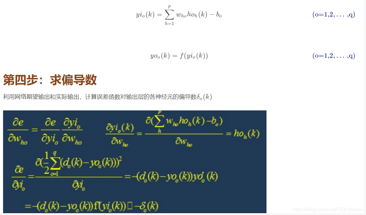
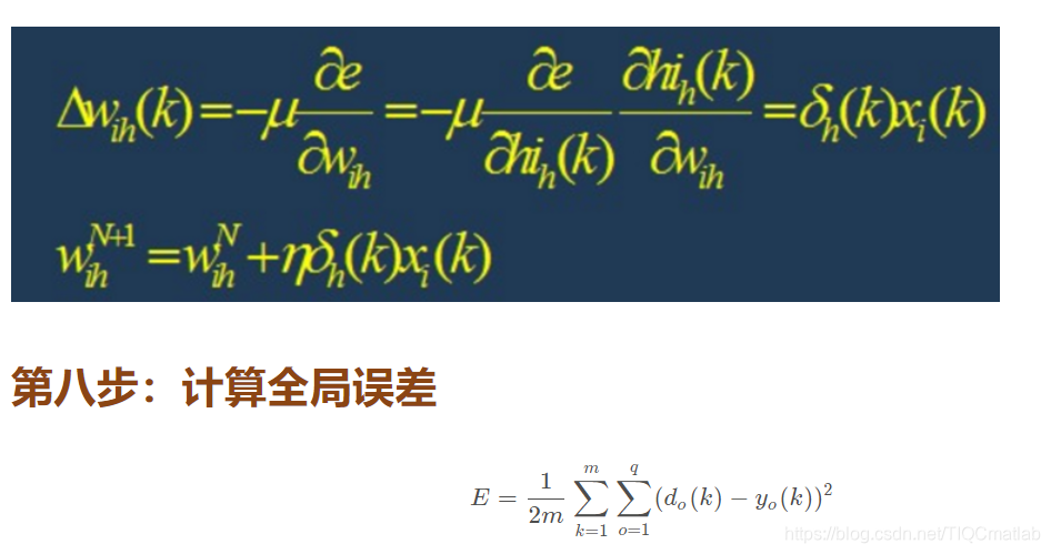
第九步：判断模型合理性
判断网络误差是否满足要求。
当误差达到预设精度或者学习次数大于设计的最大次数，则结束算法。
否则，选取下一个学习样本以及对应的输出期望，返回第三部，进入下一轮学习。

6 BP网络的设计
在进行BP网络的设计是，一般应从网络的层数、每层中的神经元个数和激活函数、初始值以及学习速率等几个方面来进行考虑，下面是一些选取的原则。
6.1 网络的层数
理论已经证明，具有偏差和至少一个S型隐层加上一个线性输出层的网络，能够逼近任何有理函数，增加层数可以进一步降低误差，提高精度，但同时也是网络 复杂化。另外不能用仅具有非线性激活函数的单层网络来解决问题，因为能用单层网络解决的问题，用自适应线性网络也一定能解决，而且自适应线性网络的 运算速度更快，而对于只能用非线性函数解决的问题，单层精度又不够高，也只有增加层数才能达到期望的结果。
6.2 隐层神经元的个数
网络训练精度的提高，可以通过采用一个隐含层，而增加其神经元个数的方法来获得，这在结构实现上要比增加网络层数简单得多。一般而言，我们用精度和 训练网络的时间来恒量一个神经网络设计的好坏：
（1）神经元数太少时，网络不能很好的学习，训练迭代的次数也比较多，训练精度也不高。
（2）神经元数太多时，网络的功能越强大，精确度也更高，训练迭代的次数也大，可能会出现过拟合(over fitting)现象。
由此，我们得到神经网络隐层神经元个数的选取原则是：在能够解决问题的前提下，再加上一两个神经元，以加快误差下降速度即可。

6.3 初始权值的选取
一般初始权值是取值在(?1,1)之间的随机数。另外威得罗等人在分析了两层网络是如何对一个函数进行训练后，提出选择初始权值量级为s√r的策略， 其中r为输入个数，s为第一层神经元个数。

6.4 学习速率
学习速率一般选取为0.01?0.8，大的学习速率可能导致系统的不稳定，但小的学习速率导致收敛太慢，需要较长的训练时间。对于较复杂的网络， 在误差曲面的不同位置可能需要不同的学习速率，为了减少寻找学习速率的训练次数及时间，比较合适的方法是采用变化的自适应学习速率，使网络在 不同的阶段设置不同大小的学习速率。

6.5 期望误差的选取
在设计网络的过程中，期望误差值也应当通过对比训练后确定一个合适的值，这个合适的值是相对于所需要的隐层节点数来确定的。一般情况下，可以同时对两个不同 的期望误差值的网络进行训练，最后通过综合因素来确定其中一个网络。

7 BP网络的局限性
BP网络具有以下的几个问题：

(1)需要较长的训练时间：这主要是由于学习速率太小所造成的，可采用变化的或自适应的学习速率来加以改进。
(2)完全不能训练：这主要表现在网络的麻痹上，通常为了避免这种情况的产生，一是选取较小的初始权值，而是采用较小的学习速率。
(3)局部最小值：这里采用的梯度下降法可能收敛到局部最小值，采用多层网络或较多的神经元，有可能得到更好的结果。

8 BP网络的改进
P算法改进的主要目标是加快训练速度，避免陷入局部极小值等，常见的改进方法有带动量因子算法、自适应学习速率、变化的学习速率以及作用函数后缩法等。 动量因子法的基本思想是在反向传播的基础上，在每一个权值的变化上加上一项正比于前次权值变化的值，并根据反向传播法来产生新的权值变化。而自适应学习 速率的方法则是针对一些特定的问题的。改变学习速率的方法的原则是，若连续几次迭代中，若目标函数对某个权倒数的符号相同，则这个权的学习速率增加， 反之若符号相反则减小它的学习速率。而作用函数后缩法则是将作用函数进行平移，即加上一个常数。

二、源代码

function varargout = Processing(varargin)
% PROCESSING MATLAB code for Processing.fig
%      PROCESSING, by itself, creates a new PROCESSING or raises the existing
%      singleton*.
%
%      H = PROCESSING returns the handle to a new PROCESSING or the handle to
%      the existing singleton*.
%
%      PROCESSING(‘CALLBACK‘,hObject,eventData,handles,...) calls the local
%      function named CALLBACK in PROCESSING.M with the given input arguments.
%
%      PROCESSING(‘Property‘,‘Value‘,...) creates a new PROCESSING or raises the
%      existing singleton*.  Starting from the left, property value pairs are
%      applied to the GUI before Processing_OpeningFcn gets called.  An
%      unrecognized property name or invalid value makes property application
%      stop.  All inputs are passed to Processing_OpeningFcn via varargin.
%
%      *See GUI Options on GUIDE‘s Tools menu.  Choose "GUI allows only one
%      instance to run (singleton)".
%
% See also: GUIDE, GUIDATA, GUIHANDLES

% Edit the above text to modify the response to help Processing

% Last Modified by GUIDE v2.5 22-May-2021 22:54:29

% Begin initialization code - DO NOT EDIT
gui_Singleton = 1;
gui_State = struct(‘gui_Name‘,       mfilename, ...
                   ‘gui_Singleton‘,  gui_Singleton, ...
                   ‘gui_OpeningFcn‘, @Processing_OpeningFcn, ...
                   ‘gui_OutputFcn‘,  @Processing_OutputFcn, ...
                   ‘gui_LayoutFcn‘,  [] , ...
                   ‘gui_Callback‘,   []);
if nargin && ischar(varargin{1})
    gui_State.gui_Callback = str2func(varargin{1});
end

if nargout
    [varargout{1:nargout}] = gui_mainfcn(gui_State, varargin{:});
else
    gui_mainfcn(gui_State, varargin{:});
end
% End initialization code - DO NOT EDIT


% --- Executes just before Processing is made visible.
function Processing_OpeningFcn(hObject, eventdata, handles, varargin)
% This function has no output args, see OutputFcn.
% hObject    handle to figure
% eventdata  reserved - to be defined in a future version of MATLAB
% handles    structure with handles and user data (see GUIDATA)
% varargin   command line arguments to Processing (see VARARGIN)

% Choose default command line output for Processing
handles.output = hObject;
setappdata(handles.Processing,‘X‘,0);
setappdata(handles.Processing,‘bw‘,0);
% Update handles structure
guidata(hObject, handles);

% UIWAIT makes Processing wait for user response (see UIRESUME)
% uiwait(handles.figure1);


% --- Outputs from this function are returned to the command line.
function varargout = Processing_OutputFcn(hObject, eventdata, handles) 
% varargout  cell array for returning output args (see VARARGOUT);
% hObject    handle to figure
% eventdata  reserved - to be defined in a future version of MATLAB
% handles    structure with handles and user data (see GUIDATA)

% Get default command line output from handles structure
varargout{1} = handles.output;


% --- Executes on button press in pushbutton12.
function pushbutton12_Callback(hObject, eventdata, handles)
% hObject    handle to pushbutton12 (see GCBO)
% eventdata  reserved - to be defined in a future version of MATLAB
% handles    structure with handles and user data (see GUIDATA)


% --- Executes on button press in pushbutton13.
function pushbutton13_Callback(hObject, eventdata, handles)
% hObject    handle to pushbutton13 (see GCBO)
% eventdata  reserved - to be defined in a future version of MATLAB
% handles    structure with handles and user data (see GUIDATA)


% --- Executes on button press in pushbutton8.
function pushbutton8_Callback(hObject, eventdata, handles)
% hObject    handle to pushbutton8 (see GCBO)
% eventdata  reserved - to be defined in a future version of MATLAB
% handles    structure with handles and user data (see GUIDATA)


% --- Executes on button press in pushbutton14.
function pushbutton14_Callback(hObject, eventdata, handles)
% hObject    handle to pushbutton14 (see GCBO)
% eventdata  reserved - to be defined in a future version of MATLAB
% handles    structure with handles and user data (see GUIDATA)


% --- Executes on button press in pushbutton15.
function pushbutton15_Callback(hObject, eventdata, handles)
% hObject    handle to pushbutton15 (see GCBO)
% eventdata  reserved - to be defined in a future version of MATLAB
% handles    structure with handles and user data (see GUIDATA)


% --- Executes on button press in pushbutton16.
function pushbutton16_Callback(hObject, eventdata, handles)
% hObject    handle to pushbutton16 (see GCBO)
% eventdata  reserved - to be defined in a future version of MATLAB
% handles    structure with handles and user data (see GUIDATA)



   
   
% --- Executes on button press in InputImage.
function InputImage_Callback(hObject, eventdata, handles)
% hObject    handle to InputImage (see GCBO)
% eventdata  reserved - to be defined in a future version of MATLAB
% handles    structure with handles and user data (see GUIDATA)

[filename,pathname]=uigetfile({‘*.jpg‘;‘*.bmp‘;‘*.tif‘;‘*.*‘},‘载入图像‘);  
 file=[pathname,filename];     
%  global S  %设置一个全局变量S，保存初始图像路径，以便之后的还原操作
%  S=file;  
 X=imread(file);  
  set(handles.imageshow1,‘HandleVisibility‘,‘ON‘); 
   axes(handles.imageshow1); 
   imshow(X);  
   handles.img=X;  
   guidata(hObject,handles); 
setappdata(handles.Processing,‘X‘,X);


% --- Executes on button press in pushbutton9.
function pushbutton9_Callback(hObject, eventdata, handles)
% hObject    handle to pushbutton9 (see GCBO)
% eventdata  reserved - to be defined in a future version of MATLAB
% handles    structure with handles and user data (see GUIDATA)


% --- Executes during object creation, after setting all properties.
function imageshow1_CreateFcn(hObject, eventdata, handles)
% hObject    handle to imageshow1 (see GCBO)
% eventdata  reserved - to be defined in a future version of MATLAB
% handles    empty - handles not created until after all CreateFcns called
% global fname fpath see
% [fname,fpath]=uigetfile(‘*.*‘,‘打开‘);
% see=[fpath fname];
% I=imread(see);
% axes(handles.axes1);
% imshow(I,‘notruesize‘);
% title(‘原始图片‘);
function B=boundaries(BW,conn,dir)
% 函数输入
% BW：二值图像矩阵%
% conn:4或8
% 返回二值图像中连通区域的边缘像素的坐标


if nargin<3   %nargin定义在用户自定义函数体内，nargin返回
              %用来调用函数的变量的个数。
    dir=‘cw‘;
end
if nargin<2
    conn=8;
end

L=bwlabel(BW,conn); %返回值是矩阵L，大小同BW，包含了BW中的连通部分的标记

% 初始化结果矩阵B 
numObjects=max(L(:));%寻找L中所作标记中的最大值，这个最大值实际上就对应着L中
% 包含的最多的连通部分的数目。
if numObjects>0
    B={zeros(0,2)};%元包数组中仅包含一个元素。
    B=repmat(B,numObjects,1);%将B进行numObjects*1个复制构成新的B。
else
    B={};
end

%在图像边界补充0值像素 
Lp=padarray(L,[1 1],0,‘both‘);

%在方向和引索坐标间建立关系 
M=size(Lp,1);%SIZE(X,1) returns the number of rows. 
             
if conn==8
    %Order is N NE E SE S SW W NW.
    offsets=[-1,M-1,M,M+1,1,-M+1,-M,-M-1];
else
    %Order is N E S W.
    offsets=[-1,M,1,-M];
end

% 搜索方向的起始方向
if conn==8
    next_search_direction_lut=[8 8 2 2 4 4 6 6];
else
    next_search_direction_lut=[4 1 2 3];
end

%下一个访问节点
if conn==8
  next_direction_lut=[2 3 4 5 6 7 8 1];
else
  next_direction_lut=[2 3 4 1];
end

START=-1;
BOUNDARY=-2;

scratch=zeros(100,1);
%Find candidate starting locations for boundaries.
[rr,cc]=find((Lp(2:end-1,:)>0)&(Lp(1:end-2,:)==0));
rr=rr+1;
for k=1:length(rr)
    r=rr(k);
    c=cc(k);
    if (Lp(r,c)>0)&(Lp(r-1,c)==0)&isempty(B{Lp(r,c)})
        %We‘ve found the start of the next boundary.Compute its linear
        %offset,record which boundary it is,mark it,and initialize the
        %counter for the number of boundary pixels.
        idx=(c-1)*size(Lp,1)+r;
        which=Lp(idx);
        scratch(1)=idx;
        Lp(idx)=START;
        numpixels=1;
        currentpixel=idx;
        initial_departure_direction=[];
        done=0;
        next_search_direction=2;
        while ~done
            %Find the next boundary pixel.
            direction=next_search_direction;
            found_next_pixel=0;
            for k=1:length(offsets)
                neighbor=currentpixel+offsets(direction);
                if Lp(neighbor)~=0
                    %Found the next boundary pixel.
                    if (Lp(currentpixel)==START)&...
                        isempty(initial_departure_direction)
                    %We are making the initial departure from the starting
                    %pixel.
                    initial_departure_direction=direction;
                    elseif (Lp(currentpixel)==START)&...
                            (initial_departure_direction==direction)
                       % We are about to retrace our path.
                       %That means we‘re done.
                       done=1;
                       found_next_pixel=1;
                       break;
                    end
                    %Take the next step along the boundary.
                    next_search_direction=...
                        next_search_direction_lut(direction);
                    found_next_pixel=1;
                    numpixels=numpixels+1;
                    if numpixels>size(scratch,1)
                        %Double the scratch space.
                        scratch(2*size(scratch,1))=0;
                    end
                    scratch(numpixels)=neighbor;
                    if Lp(neighbor)~=START
                       Lp(neighbor)=BOUNDARY;
                    end
                    currentpixel=neighbor;
                    break;
                end
                direction=next_direction_lut(direction);
            end
            if ~found_next_pixel
                %If there is no next neighbor,the object must just have a
                %single pixel.
                numpixels=2;
                scratch(2)=scratch(1);
                done=1;
            end
        end
        %Convert linear indices to row_column coordinates and save in the
        %output cell array.
        [row,col]=ind2sub(size(Lp),scratch(1:numpixels));
        B{which}=[row-1,col-1];
    end
end

if strcmp(dir,‘ccw‘)
    for k=1:length(B)
        B{k}=B{k}(end:-1:1,:);
    end
end

三、运行结果

四、备注

版本：2014a

完整代码或代写加1564658423

【树叶分类】基于matlab GUI BP神经网络植物叶片识别分类【含Matlab源码 916期】

标签：ring   偏差   形式   --   max   前馈网络   object   差值   要求   

原文地址：https://www.cnblogs.com/homeofmatlab/p/14908800.html