标签:blog http io ar os 使用 sp for strong
-----------------------------author:midu
---------------------------qq:1327706646
------------------------datetime:2014-12-08 02:29
(1)前言
以前看最小二乘,一直很模糊,后面昨天看了mit的线性代数之矩阵投影和最小二乘,突然有种豁然开朗的感觉,那位老师把他从方程的角度和矩阵联系起来,又有了不一样的理解。其实很简单就是通过找离散分布的点和贴近的直线间的最小距离,因为距离是正数,为了方便运算就加了个平方,这就是最小二乘法。然后看到了线性回归,借用网友的一片数据处理的博文做拓展。
(2)算法
这里是采用了最小二乘法计算(证明比较冗长略去)。这种方式的优点是计算简单,但是要求数据矩阵X满秩,并且当数据维数较高时计算很慢;这时候我们应该考虑使用梯度下降法或者是随机梯度下降(同Logistic回归中的思想完全一样,而且更简单)等求解。这里对估计的好坏采用了相关系数进行度量。
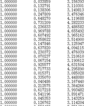
这里的txt中包含了x0的值,也就是下图中前面的一堆1,但是一般情况下我们是不给出的,也就是根据一个x预测y,这时候我们会考虑到计算的方便也会加上一个x0。
loadDataSet(fileName):
读取数据。standRegres(xArr,yArr)
普通的线性回归,这里用的是最小二乘法
![]()
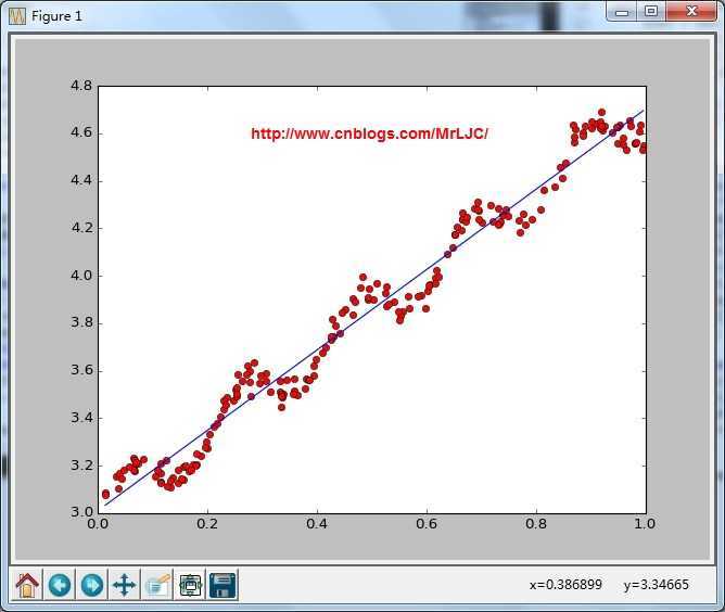
plotStandRegres(xArr,yArr,ws)
画出拟合的效果calcCorrcoef(xArr,yArr,ws)
计算相关度,用的是numpy内置的函数
结果:
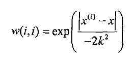
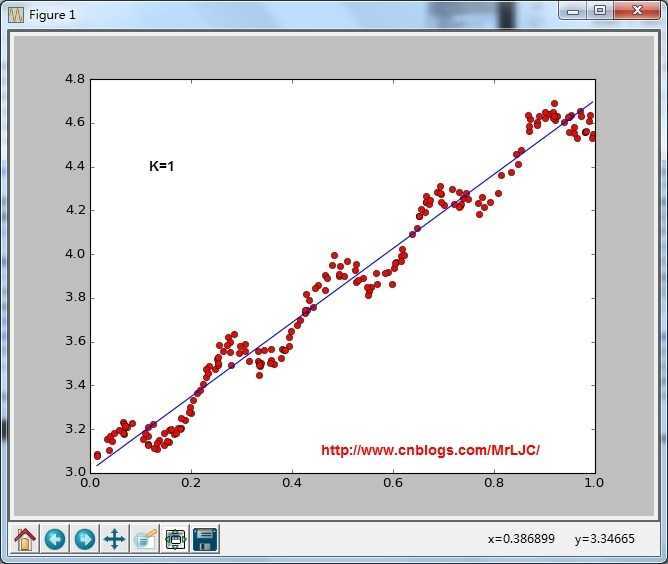
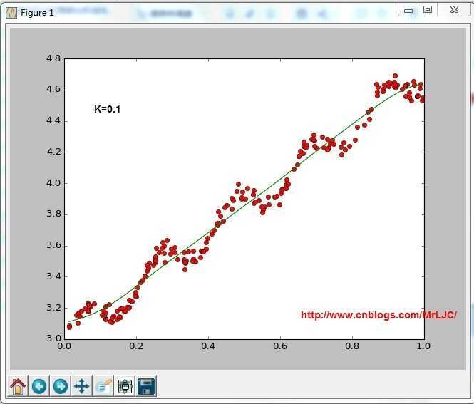
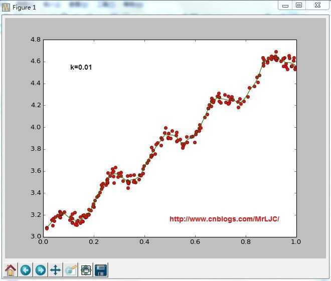
这里的想法是:我们赋予预测点附近每一个点以一定的权值,在这上面基于最小均方差来进行普通的线性回归。这里面用“核”(与支持向量机相似)来对附近的点赋予最高的权重。这里用的是高斯核:
lwlr(testPoint,xArr,yArr,k=1.0)
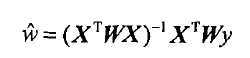
根据计算公式计算出再testPoint处的估计值,这里要给出k作为参数,k为1的时候算法退化成普通的线性回归。k越小越精确(太小可能会过拟合)求解用最小二乘法得到如下公式:
lwlrTest(testArr,xArr,yArr,k=1.0)
因为lwlr需要指定每一个点,这里把整个通过循环算出来了lwlrTestPlot(xArr,yArr,k=1.0)
将结果绘制成图像
from numpy import *
def loadDataSet(fileName):
numFeat = len(open(fileName).readline().split(‘\t‘)) - 1
dataMat = []; labelMat = []
fr = open(fileName)
for line in fr.readlines():
lineArr =[]
curLine = line.strip().split(‘\t‘)
for i in range(numFeat):
lineArr.append(float(curLine[i]))
dataMat.append(lineArr)
labelMat.append(float(curLine[-1]))
return dataMat,labelMat
def standRegres(xArr,yArr):
xMat = mat(xArr)
yMat = mat(yArr).T
xTx = xMat.T * xMat
if linalg.det(xTx) == 0.0:
print ‘This matrix is singular, cannot do inverse‘
return
ws = xTx.I * (xMat.T * yMat)
return ws
def plotStandRegres(xArr,yArr,ws):
import matplotlib.pyplot as plt
fig = plt.figure()
ax = fig.add_subplot(111)
ax.plot([i[1] for i in xArr],yArr,‘ro‘)
xCopy = xArr
print type(xCopy)
xCopy.sort()
yHat = xCopy*ws
ax.plot([i[1] for i in xCopy],yHat)
plt.show()
def calcCorrcoef(xArr,yArr,ws):
xMat = mat(xArr)
yMat = mat(yArr)
yHat = xMat*ws
return corrcoef(yHat.T, yMat)
def lwlr(testPoint,xArr,yArr,k=1.0):
xMat = mat(xArr); yMat = mat(yArr).T
m = shape(xMat)[0]
weights = mat(eye((m)))
for j in range(m):
diffMat = testPoint - xMat[j,:]
weights[j,j] = exp(diffMat*diffMat.T/(-2.0*k**2))
xTx = xMat.T * (weights * xMat)
if linalg.det(xTx) == 0.0:
print "This matrix is singular, cannot do inverse"
return
ws = xTx.I * (xMat.T * (weights * yMat))
return testPoint * ws
def lwlrTest(testArr,xArr,yArr,k=1.0):
m = shape(testArr)[0]
yHat = zeros(m)
for i in range(m):
yHat[i] = lwlr(testArr[i],xArr,yArr,k)
return yHat
def lwlrTestPlot(xArr,yArr,k=1.0):
import matplotlib.pyplot as plt
yHat = zeros(shape(yArr))
xCopy = mat(xArr)
xCopy.sort(0)
for i in range(shape(xArr)[0]):
yHat[i] = lwlr(xCopy[i],xArr,yArr,k)
fig = plt.figure()
ax = fig.add_subplot(111)
ax.plot([i[1] for i in xArr],yArr,‘ro‘)
ax.plot(xCopy,yHat)
plt.show()
#return yHat,xCopy
def rssError(yArr,yHatArr): #yArr and yHatArr both need to be arrays
return ((yArr-yHatArr)**2).sum()
def main():
#regression
xArr,yArr = loadDataSet(‘ex0.txt‘)
ws = standRegres(xArr,yArr)
print ws
#plotStandRegres(xArr,yArr,ws)
print calcCorrcoef(xArr,yArr,ws)
#lwlr
lwlrTestPlot(xArr,yArr,k=1)
if __name__ == ‘__main__‘:
main()
(3)基于bp神经网络和遗传算法,以及马尔科夫模型的实战炒股竞赛
http://www.cnblogs.com/MrLJC/p/4147697.html
http://www.cnblogs.com/qq-star/p/4148138.html
标签:blog http io ar os 使用 sp for strong
原文地址:http://www.cnblogs.com/pengkunfan/p/4150272.html