《DSP using MATLAB》示例Example 6.27

% 
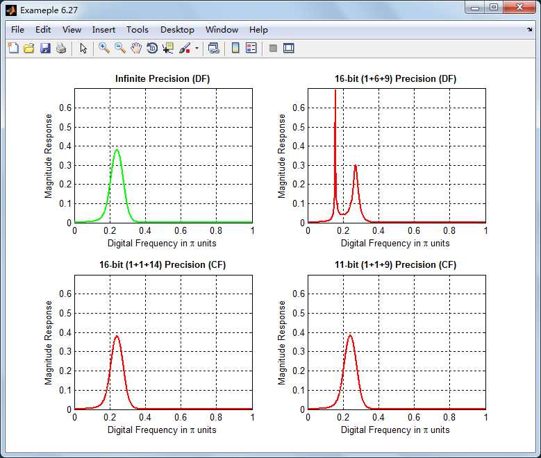
r = 0.9; theta = (pi/180)*[-55:5:-35, 35:5:55]‘;
p = r*exp(j*theta); a = poly(p); b = 1;
w = [0:500]*pi/500; H = freqz(b*1e-4, a, w);
magH = abs(H); magHdb = 20*log10(magH);

% Direct form: quantized coefficients
N = 15; [ahat, L, B] = QCoeff(a, N);
TITLE = sprintf(‘%i-bit (1+%i+%i) Precision (DF)‘, N+1, L, B);
Hhat = freqz(b*1e-4, ahat, w); magHhat = abs(Hhat);

% Cascade form: quantized coefficients: Same N
[b0, B0, A0] = dir2cas(b, a); [BAhat1, L1, B1] = QCoeff([B0, A0], N);
TITLE1 = sprintf(‘%i-bit (1+%i+%i) Precision (CF)‘, N+1, L1, B1);
Bhat1 = BAhat1(:, 1:3); Ahat1 = BAhat1(:, 4:6);
[bhat1, ahat1] = cas2dir(b0, Bhat1, Ahat1);
Hhat1 = freqz(b*1e-4, ahat1, w); magHhat1 = abs(Hhat1);

% Cascade fomr: quantized coefficients: Same B (N=L1+B)
N1 = L1 + B; [BAhat2, L2, B2] = QCoeff([B0, A0], N1);
TITLE2 = sprintf(‘%i-bit (1+%i+%i) Precision (CF)‘, N1+1, L2, B2);
Bhat2 = BAhat2(:, 1:3); Ahat2 = BAhat2(:, 4:6);
[bhat2, ahat2] = cas2dir(b0, Bhat2, Ahat2);
Hhat2 = freqz(b*1e-4, ahat2, w); magHhat2 = abs(Hhat2);


% Comparison of Magnitude Plots
Hf_1 = figure(‘paperunits‘, ‘inches‘, ‘paperposition‘, [0, 0, 6, 4]);
%figure(‘NumberTitle‘, ‘off‘, ‘Name‘, ‘Exameple 6.26a‘)
set(gcf,‘Color‘,‘white‘);

subplot(2, 2, 1); plot(w/pi, magH, ‘g‘, ‘linewidth‘, 2); axis([0, 1, 0, 0.7]);
xlabel(‘Digital Frequency in \pi units‘, ‘fontsize‘, 10);
ylabel(‘Magnitude Response‘, ‘fontsize‘, 10); grid on;
title(‘Infinite Precision (DF)‘, ‘fontsize‘, 10, ‘fontweight‘, ‘bold‘);

subplot(2, 2, 2); plot(w/pi, magHhat, ‘r‘, ‘linewidth‘, 2); axis([0, 1, 0, 0.7]);
xlabel(‘Digital Frequency in \pi units‘, ‘fontsize‘, 10);
ylabel(‘Magnitude Response‘, ‘fontsize‘, 10); grid on;
title(TITLE, ‘fontsize‘, 10, ‘fontweight‘, ‘bold‘);

subplot(2, 2, 3); plot(w/pi, magHhat1, ‘r‘, ‘linewidth‘, 2); axis([0, 1, 0, 0.7]);
xlabel(‘Digital Frequency in \pi units‘, ‘fontsize‘, 10);
ylabel(‘Magnitude Response‘, ‘fontsize‘, 10); grid on;
title(TITLE1, ‘fontsize‘, 10, ‘fontweight‘, ‘bold‘);

subplot(2, 2, 4); plot(w/pi, magHhat2, ‘r‘, ‘linewidth‘, 2); axis([0, 1, 0, 0.7]);
xlabel(‘Digital Frequency in \pi units‘, ‘fontsize‘, 10);
ylabel(‘Magnitude Response‘, ‘fontsize‘, 10); grid on;
title(TITLE2, ‘fontsize‘, 10, ‘fontweight‘, ‘bold‘);