标签:which rate str include greatest end mat 技术 sid
Q: Why might we want to use another fitting procedure instead of least squares?
A: alternative fitting procedures can yield better prediction accuracy and model interpretability.
6.1 Subset Selection
6.1.1 Best Subset Selection
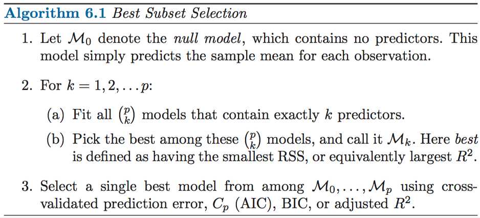
Now in order to select a single best model, we must simply choose among these p + 1 options. This task must be performed with care, because the RSS of these p + 1 models decreases monotonically, and the R-squared increases monotonically, as the number of features included in the models increases.
6.1.2 Stepwise Selection
For computational reasons, best subset selection cannot be applied with very large p. Best subset selection may also suffer from statistical problems when p is large. The larger the search space, the higher the chance of finding models that look good on the training data, even though they might not have any predictive power on future data.
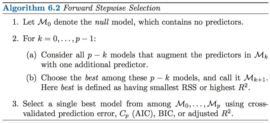
Backward stepwise selection: It begins with the full least squares model containing all p predictors, and then iteratively removes the least useful predictor.
Hybrid approach: after adding each new variable, the method may also remove any variables that no longer provide an improvement in the model fit.
6.1.3 Choosing the Optimal Model
Training set RSS and training set R2 cannot be used to select from among a set of models with different numbers of variables. Because, the training error will decrease as more variables are included in the model, but the test error may not. However, a number of techniques for adjusting the training error for the model size are available.
$$Y = \beta_0 + \beta_1X_1+...+\beta_pX_p+\epsilon (6.1)$$
Mallow‘s Cp
For a fitted least squares model containing d predictors, the Cp estimate of test MSE is computed using the equation
$$C_p = \frac{1}{n}(RSS+2d\hat \sigma^2)$$
where $\hat \sigma^{2}$ is an estimate of the variance of the error $\epsilon$ associated with each response measurement in (6.1).
Essentially, the Cp statistic adds a penalty of $2d \hat \sigma^2$ to the training RSS in order to adjust for the fact that the training error tends to underestimate the test error.
Akaike information criterion (AIC)
$$AIC= \frac{1}{n\hat\sigma^2}(RSS+2d\hat \sigma^2)$$
for least squares models, Cp and AIC are proportional to each other
Bayesian information criterion (BIC)
$$BIC= \frac{1}{n}(RSS+log(n)d\hat \sigma^2)$$
places a heavier penalty on models with many variables
Adjusted R2
$$Adjusted R^2 = 1 - \frac{RSS/(n-d-1)}{TSS/(n-1)}$$
The usual R2 is defined as 1 ? RSS/TSS
The intuition behind the adjusted R-squared is that the inclusion of unnecessary variables in the model will pay a price. To maximize Adjusted R2, we need to minimize RSS/(n-d-1)
Validation and Cross-Validation
As an alternative to the approaches just discussed, we can compute the validation set error or the cross-validation error for each model under consideration, and then select the model for which the resulting estimated test error is smallest. This procedure has an advantage relative to AIC, BIC, Cp, and adjusted R2, in that it provides a direct estimate of the test error, and makes fewer assumptions about the true underlying model. It can also be used in a wider range of model selection tasks, even in cases where it is hard to pinpoint the model degrees of freedom (e.g. the number of predictors in the model) or hard to estimate the error variance σ2.
6.2 Shrinkage Methods
We can fit a model containing all p predictors using a technique that constrains or regularizes the coefficient estimates, or equivalently, that shrinks the coefficient estimates towards zero.
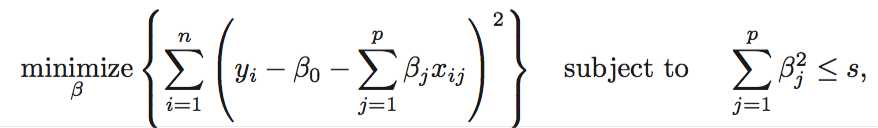
6.2.1 Ridge Regression
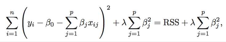
As with least squares, ridge regression seeks coefficient estimates that fit the data well, by making the RSS small. However, the second term, $\lambda \sum^{p}_{j=1}\beta_j^2$, called a shrinkage penalty, is small when β1, . . . , βp are close to zero, and so it has the effect of shrinking the estimates of βj towards zero. The tuning parameter λ serves to control the relative impact of these two terms on the regression coefficient estimates.
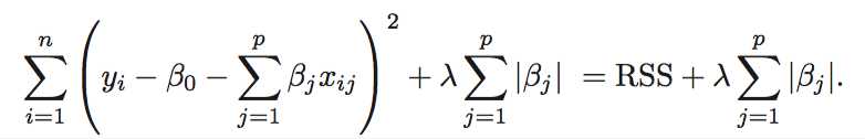
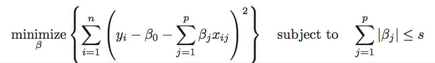
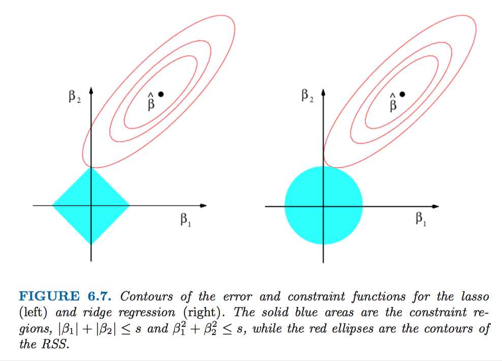
6.2.2 The Lasso
As with ridge regression, the lasso shrinks the coefficient estimates towards zero. However, in the case of the lasso, the l1 penalty has the effect of forcing some of the coefficient estimates to be exactly equal to zero when the tuning parameter λ is sufficiently large. Hence, much like best subset selection, the lasso performs variable selection. As a result, models generated from the lasso are generally much easier to interpret than those produced by ridge regression.
Another Formulation for Ridge Regression and the Lasso
6.2.3 Selecting the Tuning Parameter
Cross-validation provides a simple way to tackle this problem. We choose a grid of λ values, and compute the cross-validation error for each value of λ, as described in Chapter 5. We then select the tuning parameter value for which the cross-validation error is smallest. Finally, the model is re-fit using all of the available observations and the selected value of the tuning parameter.
6.3 Dimension Reduction Methods
The methods that we have discussed so far in this chapter are defined using the original predictors, X1, X2, . . . , Xp. We now explore a class of approaches that transform the predictors and then fit a least squares model using the transformed variables.
Let Z1, Z2, …, ZM represent M<p linear combinations of our original p predictors. That is,
$$Z_m = \sum^{p}_{j=1} \phi_{jm}X_j (6.16)$$
for some constants $\phi_{1m}$, $\phi_{2m}$ ..., $\phi_{pm}$, m = 1,...,M. We can then fit the linear regression model
$$y_i = \theta_0 + \sum^{M}_{m=1} \theta_m z_{im} + \epsilon_i$$
using least squares
The dimension of the problem has been reduced from p+1 to M +1.
6.3.1 Principal Components Regression
Principal Component Analysis(PCA) is a popular approach for deriving a low-dimensional set of features from a large set of variables.
The principal components regression (PCR) approach involves constructing the first M principal components, Z1,...,ZM, and then using these components as the predictors in a linear regression model that is fit using least squares. The key idea is that often a small number of principal components suffice to explain most of the variability in the data, as well as the relationship with the response.
It is not a feature selection method. This is because each of the M principal components used in the regression is a linear combination of all p of the original features. So PCR and ridge regression is very closedly related
6.3.2 Partial Least Squares
In the PCR approach, the directions are identified in an unsupervised way, since the response Y is not used to help determine the principal component directions. Consequently, PCR suffers from a drawback: there is no guarantee that the directions that best explain the predictors will also be the best directions to use for predicting the response.
Therefore, we now present partial least squares (PLS), a supervised alternative to PCR. Like PCR, PLS is a dimension reduction method, which first identifies a new set of features Z1,...,ZM that are linear combinations of the original features, and then fits a linear model via least squares using these M new features. But unlike PCR, PLS identifies these new features in a supervised way.
We now describe how the first PLS direction is computed. After standardizing the p predictors, PLS computes the first direction Z1 by setting each $\phi_{j1}$ in (6.16) equal to the coefficient from the simple linear regression of Y onto Xj . One can show that this coefficient is proportional to the correlation between Y and Xj. Hence, in computing Z1, PLS places the highest weight on the variables that are most strongly related to the response.
6.4 Considerations in High Dimensions
Situation: p>n
It turns out that many of the methods seen in this chapter for fitting less flexible least squares models, such as forward stepwise selection, ridge regression, the lasso, and principal components regression, are particularly useful for performing regression in the high-dimensional setting. Essentially, these approaches avoid overfitting by using a less flexible fitting approach than least squares.
Also, one should never use sum of squared errors, p-values, R2 statistics, or other traditional measures of model fit on the training data as evidence of a good model fit in the high-dimensional setting. Instead use cross-validation error.
ISL - Ch.6 Linear Model Selection and Regularization
标签:which rate str include greatest end mat 技术 sid
原文地址:http://www.cnblogs.com/sheepshaker/p/6664123.html