标签:*** amp run blog com div style number output
代码:
%% ------------------------------------------------------------------------
%%            Output Info about this m-file
fprintf(‘\n***********************************************************\n‘);
fprintf(‘        <DSP using MATLAB> Exameple 9.5 \n\n‘);

time_stamp = datestr(now, 31);
[wkd1, wkd2] = weekday(today, ‘long‘);
fprintf(‘      Now is %20s, and it is %7s  \n\n‘, time_stamp, wkd2);
%% ------------------------------------------------------------------------

n = 0:256; x = cos(pi*n); w = [0:100]*pi/100;

%% -----------------------------------------------------------------
%%                             Plot
%% -----------------------------------------------------------------
Hf1 = figure(‘units‘, ‘inches‘, ‘position‘, [1, 1, 8, 6], ...
	‘paperunits‘, ‘inches‘, ‘paperposition‘, [0, 0, 6, 4], ...
	‘NumberTitle‘, ‘off‘, ‘Name‘, ‘Exameple 9.5‘);
set(gcf,‘Color‘,‘white‘);

TF = 10;
% (a) Interpolation by I = 2, L = 5
I = 2; [y, h] = interp(x, I); H = freqz(h, 1, w); H = abs(H);
subplot(2, 2, 1);
plot(w/pi, H); axis([0, 1, 0, I+0.1]); grid on;
xlabel(‘\omega in \pi units‘); ylabel(‘Magnitude‘);
title(‘I = 2, L = 5‘, ‘fontsize‘, TF);
set(gca, ‘xtick‘, [0, 0.5, 1]);
set(gca, ‘ytick‘, [0:1:I]);

% (b) Interpolation by I = 4, L = 5
I = 4; [y, h] = interp(x, I); H = freqz(h, 1, w); H = abs(H);
subplot(2, 2, 2);
plot(w/pi, H); axis([0, 1, 0, I+0.2]); grid on;
xlabel(‘\omega in \pi units‘); ylabel(‘Magnitude‘);
title(‘I = 4, L = 5‘, ‘fontsize‘, TF);
set(gca, ‘xtick‘, [0, 0.25, 1]);
set(gca, ‘ytick‘, [0:1:I]);


% (c) Interpolation by I = 8, L = 5
I = 8; [y, h] = interp(x, I); H = freqz(h, 1, w); H = abs(H);
subplot(2, 2, 3);
plot(w/pi, H); axis([0, 1, 0, I+0.4]); grid on;
xlabel(‘\omega in \pi units‘); ylabel(‘Magnitude‘);
title(‘I = 8, L = 5‘, ‘fontsize‘, TF);
set(gca, ‘xtick‘, [0, 0.125, 1]);
set(gca, ‘ytick‘, [0:2:I]);


% (d) Interpolation by I = 8, L = 10
I = 8; [y, h] = interp(x, I, 10); H = freqz(h, 1, w); H = abs(H);
subplot(2, 2, 4);
plot(w/pi, H); axis([0, 1, 0, I+0.4]); grid on;
xlabel(‘\omega in \pi units‘); ylabel(‘Magnitude‘);
title(‘I = 8, L = 10‘, ‘fontsize‘, TF);
set(gca, ‘xtick‘, [0, 0.125, 1]);
set(gca, ‘ytick‘, [0:2:I]);
运行结果:
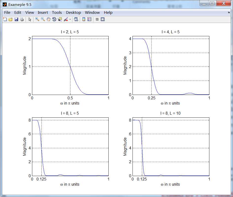
前三张图L=5,和想象的一样,滤波器是低通性质,其通带边界近似在π/I附近,并且幅度谱最大增益为I。另外注意到滤波器的过渡带和缓,
因此和理想滤波器相差较大。最后一张,L=10,和想象一样,过渡带比较陡。
任何超过L=10的情况都会导致滤波器不稳定,因此在设计过程中是必须避免的。
《DSP using MATLAB》示例Example 9.5
标签:*** amp run blog com div style number output
原文地址:http://www.cnblogs.com/ky027wh-sx/p/6901516.html