先写DTFT子函数:
function [X] = dtft(x, n, w)

%% ------------------------------------------------------------------------
%%     Computes DTFT (Discrete-Time Fourier Transform)
%%                         of Finite-Duration Sequence
%%   Note: NOT the most elegant way
%   [X] = dtft(x, n, w)
%    X  = DTFT values computed at w frequencies
%    x  = finite duration sequence over n
%    n  = sample position vector
%    w  = frequency location vector

M = 500;
k = [-M:M];                    % [-pi, pi]
%k = [0:M];                    % [0, pi]
w = (pi/M) * k;

X = x * (exp(-j*pi/M)) .^ (n‘*k);
% X = x * exp(-j*n‘*pi*k/M) ;
下面开始利用上函数开始画图。结构都一样,先显示序列x(n),在进行DTFT,画出幅度响应和相位响应。
代码:
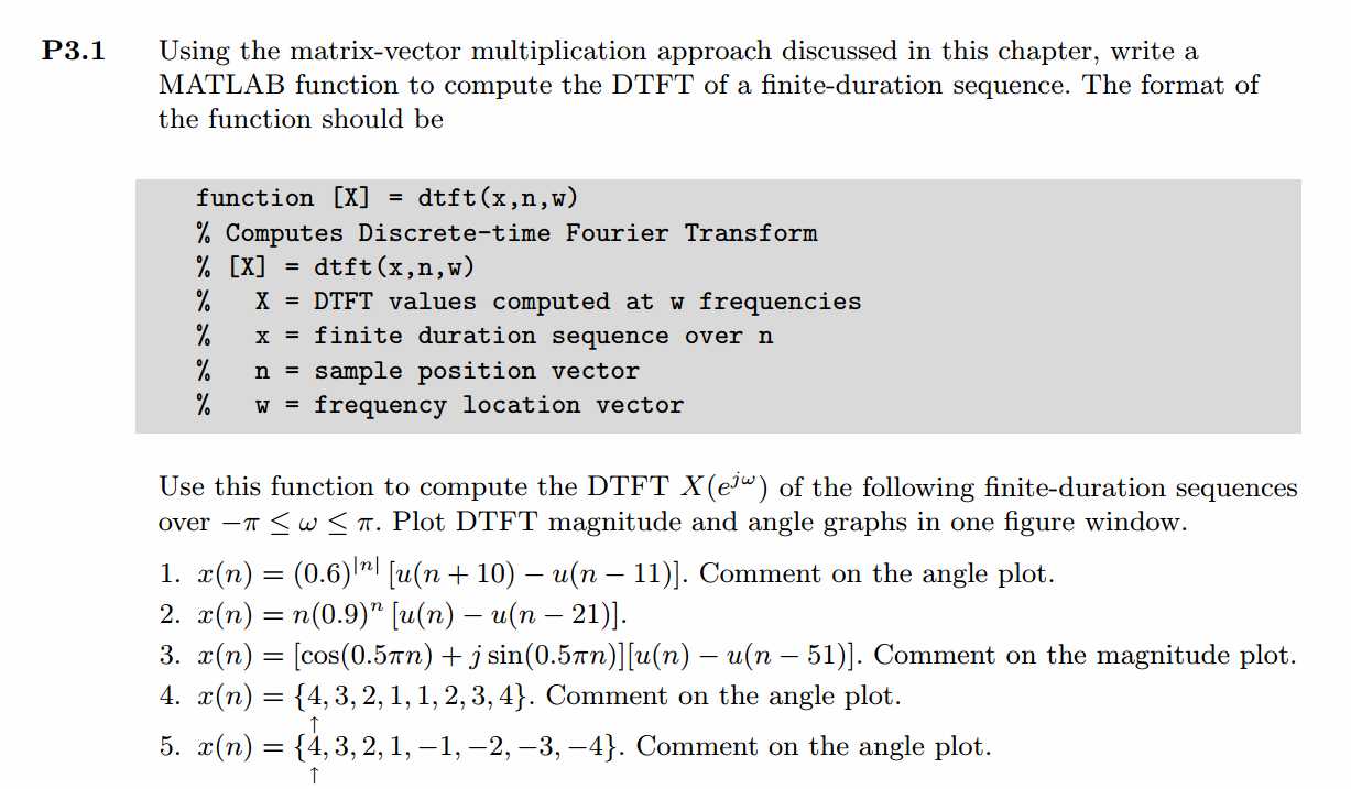
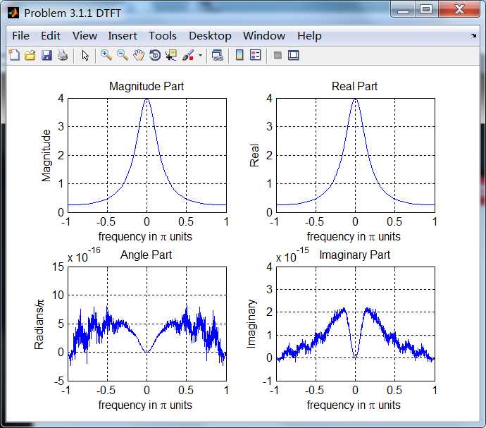
%% ------------------------------------------------------------------------
%%            Output Info about this m-file
fprintf(‘\n***********************************************************\n‘);
fprintf(‘        <DSP using MATLAB> Problem 3.1 \n\n‘);

banner();
%% ------------------------------------------------------------------------


% ----------------------------------
%            x1(n)
% ----------------------------------
n1_start = -11; n1_end = 13;
n1 = [n1_start : n1_end];

x1 = 0.6 .^ (abs(n1)) .* (stepseq(-10, n1_start, n1_end)-stepseq(11, n1_start, n1_end));

figure(‘NumberTitle‘, ‘off‘, ‘Name‘, ‘Problem 3.1 x1(n)‘);
set(gcf,‘Color‘,‘white‘);
stem(n1, x1);
xlabel(‘n‘); ylabel(‘x1‘);
title(‘x1(n) sequence‘); grid on;

M = 500;
k = [-M:M];        % [-pi, pi]
%k = [0:M];        % [0, pi]
w = (pi/M) * k;

[X1] = dtft(x1, n1, w);

magX1 = abs(X1); angX1 = angle(X1); realX1 = real(X1); imagX1 = imag(X1);

figure(‘NumberTitle‘, ‘off‘, ‘Name‘, ‘Problem 3.1 DTFT‘);
set(gcf,‘Color‘,‘white‘);
subplot(2,2,1); plot(w/pi, magX1); grid on;
title(‘Magnitude Part‘);
xlabel(‘frequency in \pi units‘); ylabel(‘Magnitude‘);
subplot(2,2,3); plot(w/pi, angX1/pi); grid on;
title(‘Angle Part‘);
xlabel(‘frequency in \pi units‘); ylabel(‘Radians/\pi‘);
subplot(‘2,2,2‘); plot(w/pi, realX1); grid on;
title(‘Real Part‘);
xlabel(‘frequency in \pi units‘); ylabel(‘Real‘);
subplot(‘2,2,4‘); plot(w/pi, imagX1); grid on;
title(‘Imaginary Part‘);
xlabel(‘frequency in \pi units‘); ylabel(‘Imaginary‘);

figure(‘NumberTitle‘, ‘off‘, ‘Name‘, ‘Problem 3.1 DTFT of x1(n)‘);;
set(gcf,‘Color‘,‘white‘);
subplot(2,1,1); plot(w/pi, magX1); grid on;
title(‘Magnitude Part‘);
xlabel(‘frequency in \pi units‘); ylabel(‘Magnitude‘);
subplot(2,1,2); plot(w/pi, angX1); grid on;
title(‘Angle Part‘);
xlabel(‘frequency in \pi units‘); ylabel(‘Radians‘);


% -------------------------------------
%            x2(n)
% -------------------------------------
n2_start = -1; n2_end = 22;
n2 = [n2_start : n2_end];

x2 = (n2 .* (0.9 .^ n2)) .* (stepseq(0, n2_start, n2_end) - stepseq(21, n2_start, n2_end));

figure(‘NumberTitle‘, ‘off‘, ‘Name‘, ‘Problem 3.1 x2(n)‘);
set(gcf,‘Color‘,‘white‘);
stem(n2, x2);
xlabel(‘n‘); ylabel(‘x2‘);
title(‘x2(n) sequence‘); grid on;


M = 500;
k = [-M:M];        % [-pi, pi]
%k = [0:M];        % [0, pi]
w = (pi/M) * k;

[X2] = dtft(x2, n2, w);

magX2 = abs(X2); angX2 = angle(X2); realX2 = real(X2); imagX2 = imag(X2);

figure(‘NumberTitle‘, ‘off‘, ‘Name‘, ‘Problem 3.1 DTFT of x2(n)‘);;
set(gcf,‘Color‘,‘white‘);
subplot(2,1,1); plot(w/pi, magX2); grid on;
title(‘Magnitude Part‘);
xlabel(‘frequency in \pi units‘); ylabel(‘Magnitude‘);
subplot(2,1,2); plot(w/pi, angX2); grid on;
title(‘Angle Part‘);
xlabel(‘frequency in \pi units‘); ylabel(‘Radians‘);


% -------------------------------------
%            x3(n)
% -------------------------------------
n3_start = -1; n3_end = 52;
n3 = [n3_start : n3_end];

x3 = (cos(0.5*pi*n3) + j * sin(0.5*pi*n3)) .* (stepseq(0, n3_start, n3_end) - stepseq(51, n3_start, n3_end));

figure(‘NumberTitle‘, ‘off‘, ‘Name‘, ‘Problem 3.1 x3(n)‘);
set(gcf,‘Color‘,‘white‘);
stem(n3, x3);
xlabel(‘n‘); ylabel(‘x3‘);
title(‘x3(n) sequence‘); grid on;

M = 500;
k = [-M:M];        % [-pi, pi]
%k = [0:M];        % [0, pi]
w = (pi/M) * k;

[X3] = dtft(x3, n3, w);

magX3 = abs(X3); angX3 = angle(X3); realX3= real(X3); imagX3 = imag(X3);

figure(‘NumberTitle‘, ‘off‘, ‘Name‘, ‘Problem 3.1 DTFT of x3(n)‘);;
set(gcf,‘Color‘,‘white‘);
subplot(2,1,1); plot(w/pi, magX3); grid on;
title(‘Magnitude Part‘);
xlabel(‘frequency in \pi units‘); ylabel(‘Magnitude‘);
subplot(2,1,2); plot(w/pi, angX3); grid on;
title(‘Angle Part‘);
xlabel(‘frequency in \pi units‘); ylabel(‘Radians‘);


% -------------------------------------
%            x4(n)
% -------------------------------------
n4_start = 0; n4_end = 7;
n4 = [n4_start : n4_end];

x4 = [4:-1:1, 1:4];

figure(‘NumberTitle‘, ‘off‘, ‘Name‘, ‘Problem 3.1 x4(n)‘);
set(gcf,‘Color‘,‘white‘);
stem(n4, x4, ‘r‘, ‘filled‘);
xlabel(‘n‘); ylabel(‘x4‘);
title(‘x4(n) sequence‘); grid on;

M = 500;
k = [-M:M];        % [-pi, pi]
%k = [0:M];        % [0, pi]
w = (pi/M) * k;

[X4] = dtft(x4, n4, w);

magX4 = abs(X4); angX4 = angle(X4); realX4= real(X4); imagX4 = imag(X4);

figure(‘NumberTitle‘, ‘off‘, ‘Name‘, ‘Problem 3.1 DTFT of x3(n)‘);;
set(gcf,‘Color‘,‘white‘);
subplot(2,1,1); plot(w/pi, magX4); grid on;
title(‘Magnitude Part‘);
xlabel(‘frequency in \pi units‘); ylabel(‘Magnitude‘);
subplot(2,1,2); plot(w/pi, angX4); grid on;
title(‘Angle Part‘);
xlabel(‘frequency in \pi units‘); ylabel(‘Radians‘);


% -------------------------------------
%            x5(n)
% -------------------------------------
n5_start = 0; n5_end = 7;
n5 = [n5_start : n5_end];

x5 = [4:-1:1, -1:-1:-4];

figure(‘NumberTitle‘, ‘off‘, ‘Name‘, ‘Problem 3.1 x5(n)‘);
set(gcf,‘Color‘,‘white‘);
stem(n5, x5, ‘r‘, ‘filled‘);
xlabel(‘n‘); ylabel(‘x5‘);
title(‘x5(n) sequence‘); grid on;

M = 500;
k = [-M:M];        % [-pi, pi]
%k = [0:M];        % [0, pi]
w = (pi/M) * k;

[X5] = dtft(x5, n5, w);

magX5 = abs(X5); angX5 = angle(X5); realX5= real(X5); imagX5 = imag(X5);

figure(‘NumberTitle‘, ‘off‘, ‘Name‘, ‘Problem 3.1 DTFT of x5(n)‘);
set(gcf,‘Color‘,‘white‘);
subplot(2,1,1); plot(w/pi, magX5); grid on;
title(‘Magnitude Part‘);
xlabel(‘frequency in \pi units‘); ylabel(‘Magnitude‘);
subplot(2,1,2); plot(w/pi, angX5); grid on;
title(‘Angle Part‘);
xlabel(‘frequency in \pi units‘); ylabel(‘Radians‘);
运行结果:
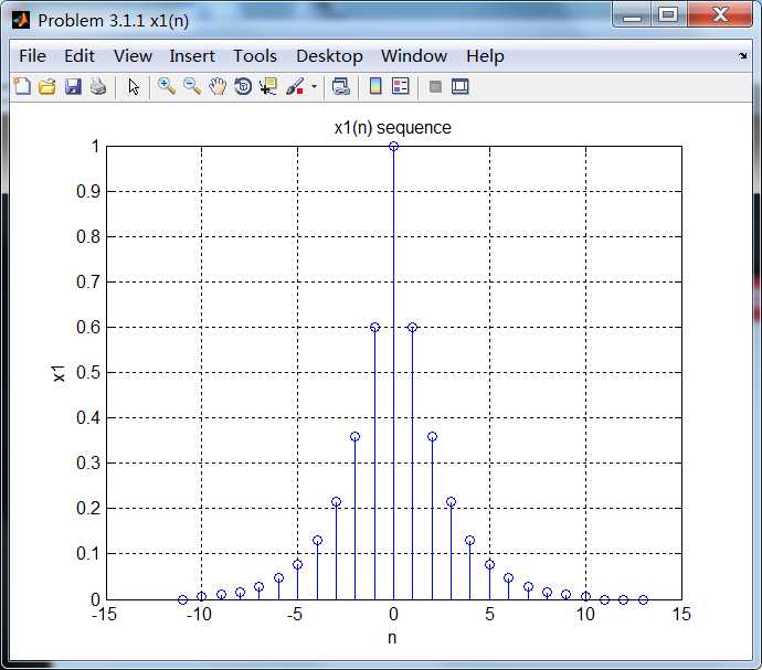
相位响应是关于ω=0偶对称的。
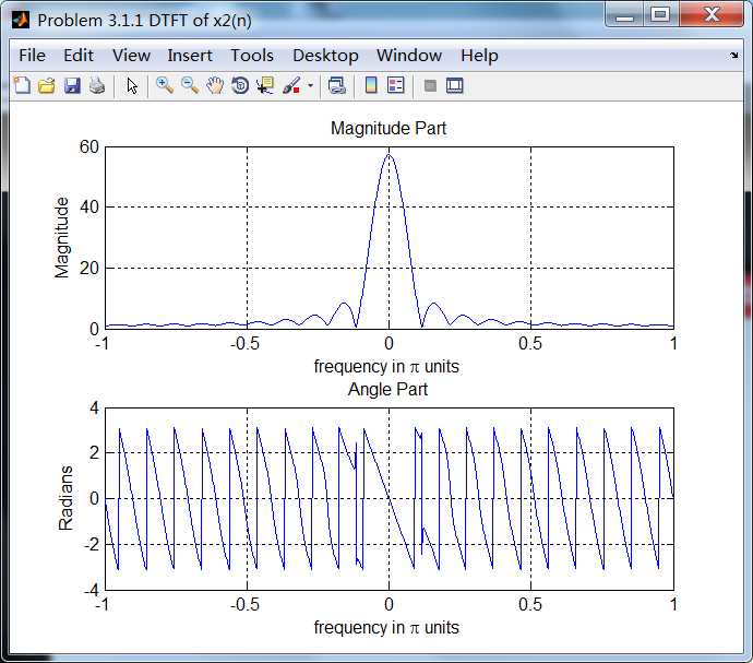
序列2:
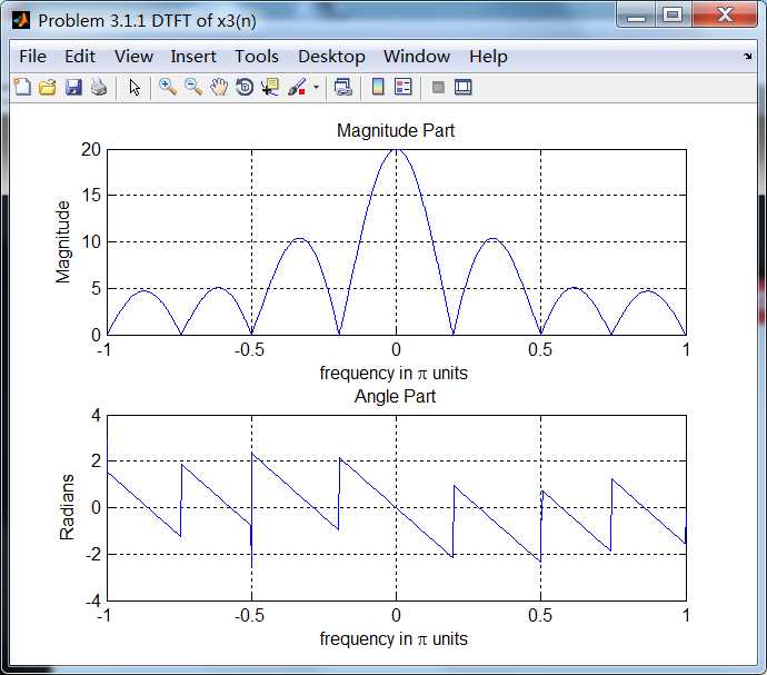
序列3:
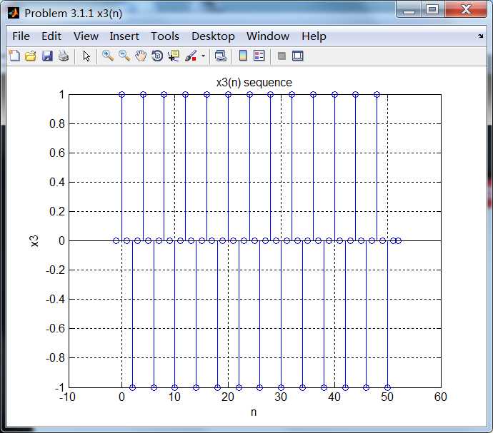
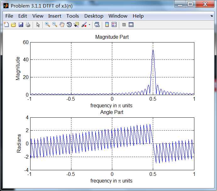
序列3的主要频率分量位于ω=0.5π。
序列4:
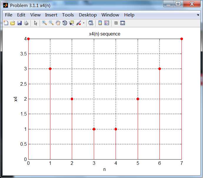
序列4的相位谱关于ω= 0奇对称。
序列5:
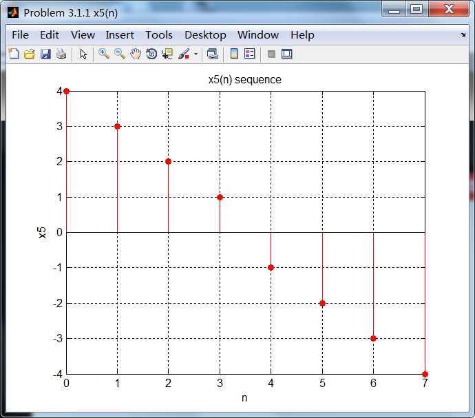
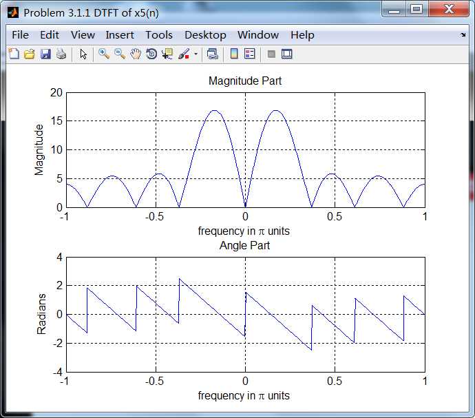
序列5的相位谱关于ω=0奇对称。