标签:iter 作业 pyplot 向量 code load 一个 flat 导致
前言:今天从早上开始写吴恩达多层神经网络的题目。反复运算,出现一个天坑,一个存储矩阵的字典parameters的W1和b1在传入函数updata_parameters前维数还是(7, 12288), 传进去后变成了(3, 4)导致不能和grads["dW1"]的维数(7, 12288)进行广播出错。调了半天也不知道到底哪里出错了。最后重新写了一遍没有出错。
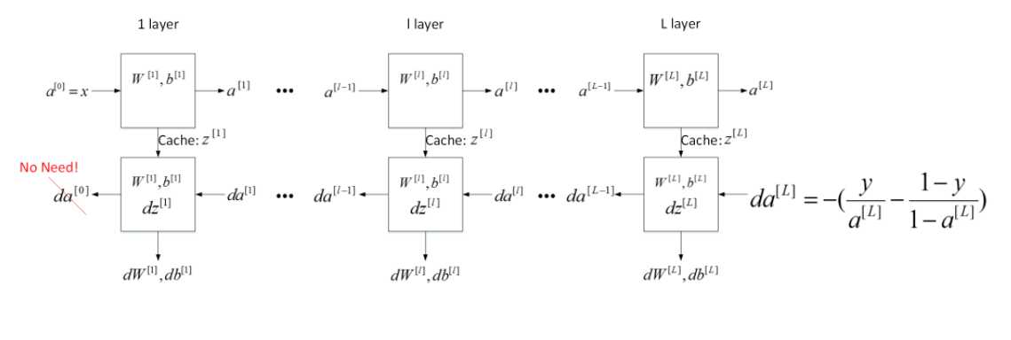
神经网络训练过程:
1.初始化参数
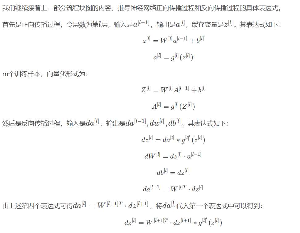
2.进行前向传播(其中分两部分,一部分是前向传播的计算部分,另一部分是前向传播的激活部分)
3.计算损失
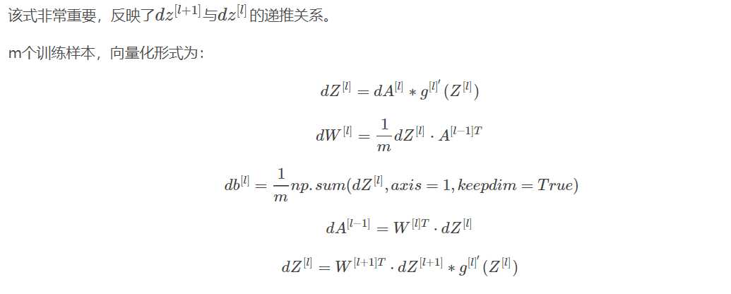
4.进行后向传播(同样分为两部分,一部分是后向传播的计算部分,另一部分是后向传播的激活部分)
5.更新参数,整合模型,进行预测
1.初始化参数
首先导入需要用到的包。我们先做只有两层的神经网络。
 1 import numpy as np
 2 import h5py
 3 import matplotlib.pyplot as plt
 4 import testCase
 5 from dnn_utils import sigmoid, sigmoid_backward, relu, relu_backward
 6 import lr_utils
 7
 8
 9 plt.rcParams[‘figure.figsize‘] = (5.0, 4.0);
10 plt.rcParams[‘image.interpolation‘] = ‘nearest‘;
11 plt.rcParams[‘image.cmap‘] = ‘gray‘;
12
13
14 np.random.seed(1);#初始化随机种子
进行参数的初始化。
 1 def initialize_parameters(n_x, n_h, n_y):#因为只有两层,所以只有输入层数量n_x,隐藏层数量n_h,输出层数量n_y
 2     np.random.seed(1);
 3
 4     W1 = np.random.randn(n_h, n_x) * 0.01;
 5     b1 = np.zeros((n_h, 1));
 6     W2 = np.random.randn(n_y, n_h) * 0.01;
 7     b2 = np.zeros((n_y, 1));
 8
 9     assert(W1.shape == (n_h, n_x));
10     assert(b1.shape == (n_h, 1));
11     assert(W2.shape == (n_y, n_h));
12     assert(b2.shape == (n_y, 1));
13
14     parameters = {"W1": W1,
15                   "b1": b1,
16                   "W2": W2,
17                   "b2": b2};
18
19     return parameters;
2.进行前向传播
进行前向传播的计算部分,计算Z,需要传入的参数为A,W,b, 并将A,W,b放入缓存cache中,后面需要用到。
1 def linear_forward(A, W, b):
2
3     Z = np.dot(W, A) + b;
4
5     assert(Z.shape == (W.shape[0], A.shape[1]));
6     cache = (A, W, b);
7
8     return Z, cache;
接着计算前向传播的激活部分,需要传入的数据是A_prev(前一层的激活值A),W, b,激活函数的类型activation。
 1 def linear_activation_forward(A_prev, W, b, activation):
 2     if activation == "sigmoid":
 3         Z, linear_cache = linear_forward(A_prev, W, b); # Z, linear_cache中缓存(W, A_prev, B)
 4         A, activation_cache = sigmoid(Z); # A, activation_cache中缓存(Z)
 5     elif activation == "relu":
 6         Z, linear_cache = linear_forward(A_prev, W, b);
 7         A, activation_cache = relu(Z);
 8
 9     assert (A.shape == (W.shape[0], A_prev.shape[1]));
10     cache = (linear_cache, activation_cache); #, ((W, A_prev, B) ,(Z))
11
12     return A, cache;
3.计算损失
需要传入的参数是最后第L层的激活值AL,和目标向量Y。
1 def compute_cost(AL, Y):
2     m = Y.shape[1];
3
4     cost = -1 / m * (np.dot(Y, np.log(AL).T) + np.dot(1 - Y, np.log(1 - AL).T));
5
6     cost = np.squeeze(cost);      # 将形状如[[17]]的向量转为形状为17的向量
7     assert(cost.shape == ());
8
9     return cost;
4.后向传播
先计算后向传播的计算部分。需要的参数是dZ(可以通过dA和Z计算得出), cache中缓存的是(A_prev, W, b)。
 1 def linear_backward(dZ, cache):
 2     A_prev, W, b = cache;
 3     m = A_prev.shape[1];
 4
 5     dW = 1 / m * np.dot(dZ, A_prev.T);
 6     db = 1 / m * np.sum(dZ, axis = 1, keepdims = True);
 7     dA_prev = np.dot(W.T, dZ);
 8
 9     assert (dA_prev.shape == A_prev.shape);
10     assert (dW.shape == W.shape);
11     assert (db.shape == b.shape);
12
13     return dA_prev, dW, db;
接着计算后向传播的激活部分。需要的参数是dA, cache(有两部分缓存的值,一个是linear_cache,一个是activation_cache), activation。
 1 def linear_activation_backward(dA, cache, activation):
 2
 3     linear_cache, activation_cache = cache
 4
 5     if activation == "relu":
 6         dZ = relu_backward(dA, activation_cache);
 7         dA_prev, dW, db = linear_backward(dZ, linear_cache);
 8
 9     elif activation == "sigmoid":
10         dZ = sigmoid_backward(dA, activation_cache);
11         dA_prev, dW, db = linear_backward(dZ, linear_cache);
12
13     return dA_prev, dW, db;
5.更新参数,整合模型,进行预测
更新参数需要传入的参数有parameters(存储参数W1, b1等的字典), grads(存储梯度的字典), learning_rate。
1 def update_parameters(parameters, grads, learning_rate):
2     L = len(parameters) // 2 #整除2,因为parameters中的参数是按W1,b1,W2,b2排列的
3     for l in range(L):
4         parameters["W" + str(l + 1)] -= learning_rate * grads["dW" + str(l + 1)];
5         parameters["b" + str(l + 1)] -= learning_rate * grads["db" + str(l + 1)];
6     return parameters;
传入吴恩达第二周编程作业中的数据集。
1 train_set_x_orig , train_set_y , test_set_x_orig , test_set_y , classes = lr_utils.load_dataset()
2
3 train_x_flatten = train_set_x_orig.reshape(train_set_x_orig.shape[0], -1).T
4 test_x_flatten = test_set_x_orig.reshape(test_set_x_orig.shape[0], -1).T
5
6 train_x = train_x_flatten / 255
7 train_y = train_set_y
8 test_x = test_x_flatten / 255
9 test_y = test_set_y
整合模型。
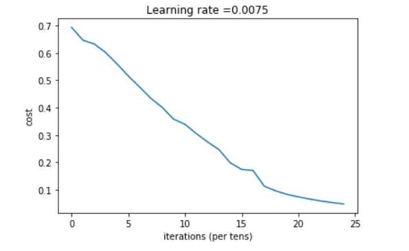
 1 def two_layer_model(X, Y, layers_dims, learning_rate = 0.0075, num_iterations = 3000, print_cost=False):
 2
 3     np.random.seed(1);
 4     grads = {};
 5     costs = [];
 6     m = X.shape[1];
 7     (n_x, n_h, n_y) = layers_dims;
 8
 9     parameters = initialize_parameters(n_x, n_h, n_y);
10
11     W1 = parameters["W1"];
12     b1 = parameters["b1"];
13     W2 = parameters["W2"];
14     b2 = parameters["b2"];
15
16
17     for i in range(0, num_iterations):
18         A1, cache1 = linear_activation_forward(X, W1, b1, "relu");
19         A2, cache2 = linear_activation_forward(A1, W2, b2, "sigmoid");
20
21         cost = compute_cost(A2, Y);
22
23         dA2 = - (np.divide(Y, A2) - np.divide(1 - Y, 1 - A2));
24
25         dA1, dW2, db2 = linear_activation_backward(dA2, cache2, "sigmoid");
26         dA0, dW1, db1 = linear_activation_backward(dA1, cache1, "relu");
27
28         grads[‘dW1‘] = dW1;
29         grads[‘db1‘] = db1;
30         grads[‘dW2‘] = dW2;
31         grads[‘db2‘] = db2;
32
33         parameters = update_parameters(parameters, grads, learning_rate);
34
35         W1 = parameters["W1"];
36         b1 = parameters["b1"];
37         W2 = parameters["W2"];
38         b2 = parameters["b2"];
39
40         if i % 100 == 0:
41             #记录成本
42             costs.append(cost)
43             #是否打印成本值
44             if print_cost:
45                 print("第", i ,"次迭代,成本值为:" ,np.squeeze(cost))
46
47
48     plt.plot(np.squeeze(costs));
49     plt.ylabel(‘cost‘);
50     plt.xlabel(‘iterations (per tens)‘);
51     plt.title("Learning rate =" + str(learning_rate));
52     plt.show();
53
54     return parameters;
整合完成后直接调用该函数就可以进行训练。
1 n_x = 12288
2 n_h = 7
3 n_y = 1
4 parameters = two_layer_model(train_x, train_y, layers_dims = (n_x, n_h, n_y), num_iterations = 2500, print_cost = True);
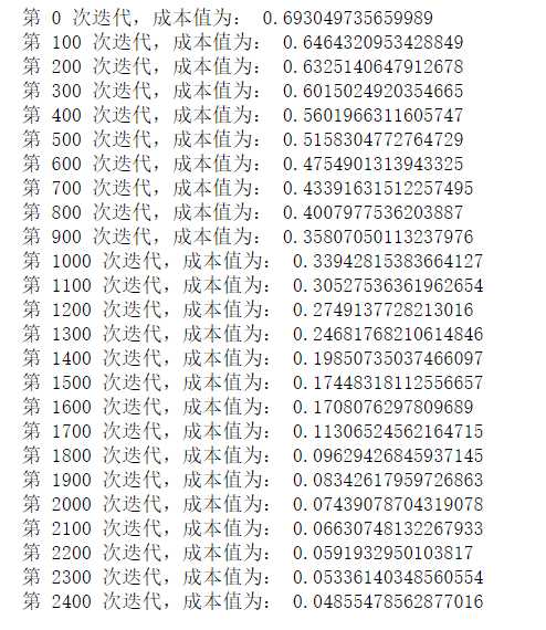
训练结果:
查看一下准确率,需要写一个函数。
 1 def predict(X, y, parameters):
 2     m = X.shape[1]
 3     n = len(parameters) // 2 # 神经网络的层数
 4     p = np.zeros((1,m))
 5
 6     #根据参数前向传播
 7     probas, caches = L_model_forward(X, parameters)
 8
 9     for i in range(0, probas.shape[1]):
10         if probas[0,i] > 0.5:
11             p[0,i] = 1
12         else:
13             p[0,i] = 0
14
15     print("准确度为: "  + str(float(np.sum((p == y))/m)))
16
17     return p
查看准确率。
1 pred_train = predict(train_x, train_y, parameters) #训练集
2 pred_test = predict(test_x, test_y, parameters) #测试集
![]()
相较之前的logistic回归的预测70%有所提高。
标签:iter 作业 pyplot 向量 code load 一个 flat 导致
原文地址:https://www.cnblogs.com/1-0001/p/12057501.html