Derivative Pricing_2_Vasicek

标签：euler   sam   mic   type   comm   zed   mat   rom   run   

*Catalog

1. Plotting Vasicek Trajectories

2. CKLS Method for Parameter Estimation (elaborated by GMM and Euler Approx)

3. Application

1. Plotting Vasicek Trajectories

　　(1) Basic outlooking:

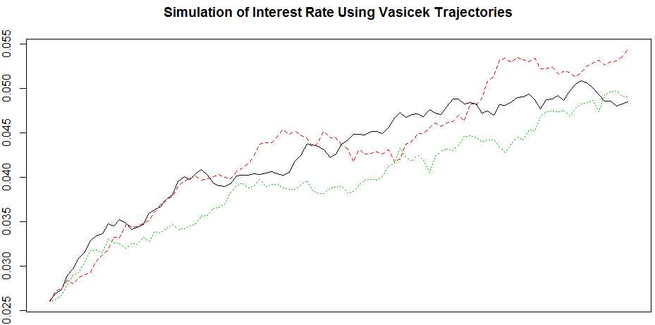
vasicek <- function(alpha, beta, sigma, n = 100, r0 = 0.026) {
        v <- rep(0, n)
        v[1] <- r0
        for (i in 2:n) {
                v[i] <- v[i - 1] + alpha * (beta - v[i - 1]) + sigma * rnorm(1)
        }
        return(v)
}
set.seed(13)
r <- replicate(3, vasicek(0.02, 0.056, 0.0006))
# plot columns of matrix against columns of another matrix
matplot(r, type = ‘l‘, ylab = ‘‘, xlab = ‘Time‘, xaxt = ‘no‘,
        main = ‘Simulation of Interest Rate Using Vasicek Trajectories‘)
lines(c(-1, 101), c(0.056, 0.056), col = ‘grey‘, lwd = 2, lty = 1)

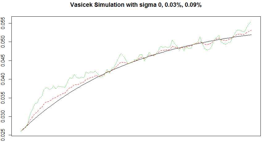
　　(2) Characteristics:

# change sigma (old sigma is 0.0006)
r <- sapply(c(0, 0.0003, 0.0009),
            function(sigma){
                    set.seed(23); vasicek(0.02, 0.056, sigma)
            })
matplot(r, type = ‘l‘, ylab = ‘‘, xlab = ‘Time‘, xaxt = ‘no‘,
        main = ‘Vasicek Simulation with sigma 0, 0.03%, 0.09%‘)

# change alpha (old alpha is 0.02)
r <- sapply(c(0.002, 0.02, 0.2),
            function(alpha){
                    set.seed(33); vasicek(alpha, 0.056, 0.0006)
            })
matplot(r, type = ‘l‘, ylab = ‘‘, xlab = ‘Time‘, xaxt = ‘no‘,
        main = ‘Vasicek Simulation with alpha 0.2%, 2%, 20%‘)

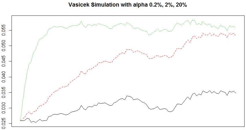
　　(3) Comments:

　　　　This model is a continuous, affine and one-factor stochastic interest rate model.

　　　　It follows a mean-reverting process (expected value converges to beta when Time of alpha goes to infinity (alpha can be treated as speed of adjustment to the 　　　　long-run beta). The higher alpha, the earlier reach long-term beta (which input by me as 0.056). As alpha goes infinity, variance converges to 0.

2. Parameter Estimation

　　(1) Generalized Method of Moments:

　　　　gamma = 0 in Vasicek model;

　　　　gamma = 0.5 in CIR model (which assumes that volatility term proportional to the square root of the interest rate level; and that interest rate has non-central

　　　　 chi-squared distribution);

　　(2) Mechanism:

　　　　Denote a vector of parameters to be estimated, theta = (alpha, beta, sigma, gamma);

　　　　Set null hypothesis is : E[ M_t(theta) ] = 0;

　　　　Use a sample corresponding to E[ M_t(theta) ], which is denoted as m_t(theta) = (1/n) * Σ M_t(theta), where t from 1 to n, and n is number of observations;

　　　　Introduce omega as a weight matrix, which is symmetric, positive and definite;

　　　　Thus, GMM minimize this quadratic term: m_t(theta)Ω(theta)m_t(theta);

3. Application 

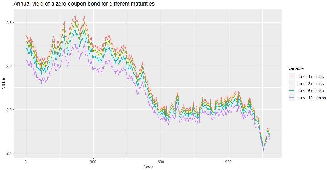
　　(1) Simulate bond prices with different maturities:

library(SMFI5)
a <- bond.vasicek(alpha = 0.5, beta = 2.55, sigma = 0.365, q1 = 0.3, q2 = 0,
            r0 = 3.5, n = 1080, maturities = c(1/12, 3/12, 6/12, 1), days = 365)
plot(a)

Derivative Pricing_2_Vasicek

标签：euler   sam   mic   type   comm   zed   mat   rom   run   

原文地址：https://www.cnblogs.com/sophhhie/p/12284577.html