标签:ssi 图片 inline otherwise 它的 好处 load function diff
C51算法理论上用Wasserstein度量衡量两个累积分布函数间的距离证明了价值分布的可行性,但在实际算法中用KL散度对离散支持的概率进行拟合,不能作用于累积分布函数,不能保证Bellman更新收敛;且C51算法使用价值分布的若干个固定离散支持,通过调整它们的概率来构建价值分布。
而分位数回归(quantile regression)的distributional RL对此进行了改进。首先,使用了C51的“转置”,即固定若干个离散支持的均匀概率,调整离散支持的位置;引入分位数回归的思想,近似地实现了Wasserstein距离作为损失函数。
假设\(\mathcal{Z}_Q\)是分位数分布空间,可以将它的累积概率函数均匀分为\(N\)等分,即\(\tau_0,\tau_1...,\tau_N(\tau_i=\frac{i}{N},i=0,1,..,N)\)。使用模型\(\theta:\mathcal{S}\times \mathcal{A}\to \mathbb{R}^N\)来预测分位数分布\(Z_\theta \in \mathcal{Z}_Q\),即模型\(\{\theta_i (s,a)\}\)将状态-动作对\((s,a)\)映射到均匀概率分布上。\(Z_\theta (s,a)\)的定义如下
其中,\(\delta_z\)表示在\(z\in\mathbb{R}\)处的Dirac函数
与C51算法相比,这种做法的好处:
使用1-Wassertein距离对随机价值分布\(Z\in \mathcal{Z}\)到\(\mathcal{Z}_Q\)的投影进行量化:
假设\(Z_\theta\)的支持集为\(\{\theta_1,...,\theta_N \}\),那么
其中,\(\tau_i,\tau_{i-1}\in[0,1]\)。论文指出,当\(F_Z^{-1}\)是逆累积分布函数时,\(F_Z^{-1}((\tau_{i-1}+\tau_i)/2)\)最小。因此,量化中点为\(\mathcal{\hat\tau_i}=\frac{\tau_{i-1}+\tau_i}{2}(1\le i\le N)\),且最小化\(W_1\)的支持\(\theta_i=F_Z^{-1}(\mathcal{\hat\tau_i})\)。如下图
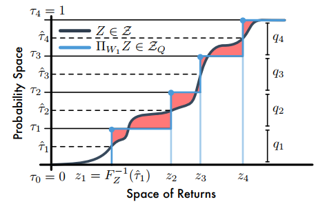
【注】C51是将回报空间(横轴)均分为若干个支持,然后求Bellman算子更新后回报落在每个支持上的概率,而分位数投影是将累积概率(纵轴)分为若干个支持(图中是4个支持),然后求出对应每个支持的回报值;图中阴影部分的面积和就是1-Wasserstein误差。
建立分位数投影后,需要去近似分布的分位数函数,需要引入分位数回归损失。对于分布\(Z\)和一个给定的分位数\(\tau\),分位数函数\(F_Z^{-1}(\tau)\)的值可以通过最小化分位数回归损失得到
最终,整体的损失函数为
但是,分位数回归损失在0处不平滑。论文进一步提出了quantile Huber loss:
QRTD算法(quantile regression temporal difference learning algorithm)的更新
\(a\sim\pi (\cdot|s),r\sim R(s,a),s^\prime\sim P(\cdot|s,a),z^\prime\sim Z_\theta(s^\prime)\)
其中,\(Z_\theta\)是由公式(1)给出的分位数分布,\(\theta_i (s)\)是状态\(s\)下\(F_{Z^\pi (s)}^{-1}(\mathcal{\hat \tau}_i)\)的估计值。
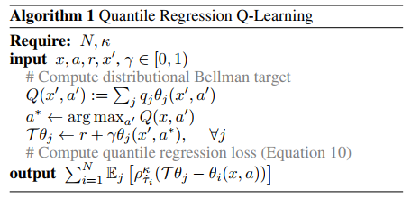
QR-DQN算法伪代码
1. Dirac Delta Function
Will Dabney, Mark Rowland, Marc G. Bellemare, Rémi Munos. Distributional Reinforcement Learning with Quantile Regression. 2017.
Distributional RL
3. Distributional Reinforcement Learning with Quantile Regression
标签:ssi 图片 inline otherwise 它的 好处 load function diff
原文地址:https://www.cnblogs.com/HughCai/p/13862526.html