标签:blur skin digital http contain 算子 load one 差分
上一部分介绍的blur能够将图片模糊化, 这部分介绍的是突出图片的边缘的细节.
什么是边缘呢? 往往是像素点跳跃特别大的点, 这部分和梯度的概念是类似的, 可以如下定义图片的一阶导数而二阶导数:
注: 或许用差分来表述更为贴切.
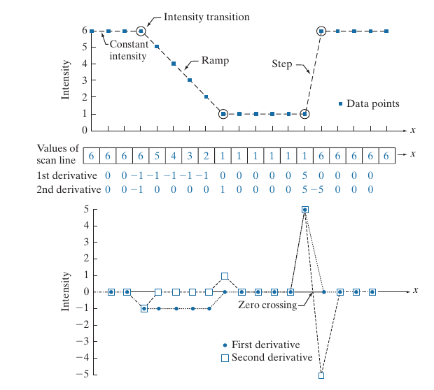
如上图实例所示, 描述了密度值沿着\(x\)的变化, 一阶导数似乎能划分区域, 而二阶导数能够更好的“识别"边缘.
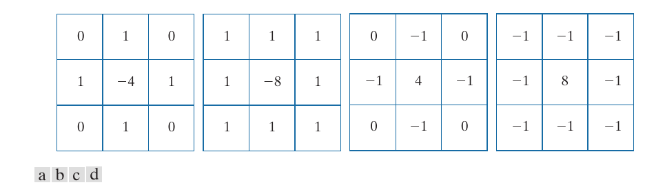
著名的laplacian算子:
在digital image这里:
这个算子用kernel表示是下面的(a), 但是在实际中也有(b, c, d)的用法, (b, d)额外用到了对角的信息, 注意到这些kernels都满足
最后
\(c=-1\), 如果a, b, \(c=1\)如果c, d.
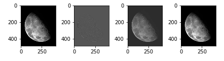
kernel = -np.ones((3, 3))
kernel[1, 1] = 8
laps = cv2.filter2D(img, -1, kernel)
laps = (laps - laps.min()) / (laps.max() - laps.min()) * 255
img_pos = img + laps
img_neg = img - laps
fig, axes = plt.subplots(1, 4)
axes[0].imshow(img, cmap=‘gray‘)
axes[1].imshow(laps, cmap=‘gray‘)
axes[2].imshow(img_pos, cmap=‘gray‘)
axes[3].imshow(img_neg, cmap=‘gray‘)
plt.tight_layout()
plt.show()
kernel = np.ones((3, 3))
kernel[0, 0] = 0
kernel[0, 2] = 0
kernel[1, 1] = -4
kernel[2, 0] = 0
kernel[2, 2] = 0
laps = cv2.filter2D(img, -1, kernel)
laps = (laps - laps.min()) / (laps.max() - laps.min()) * 255
img_pos = img + laps
img_neg = img - laps
fig, axes = plt.subplots(1, 4)
axes[0].imshow(img, cmap=‘gray‘)
axes[1].imshow(laps, cmap=‘gray‘)
axes[2].imshow(img_pos, cmap=‘gray‘)
axes[3].imshow(img_neg, cmap=‘gray‘)
plt.tight_layout()
plt.show()
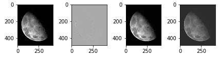
有点奇怪... 注意到我上面对laps进行标准化处理了, 如果没这个处理其实感觉是差不多的\(c=1,-1\).
注意到, 之前的box kernel,
考虑\(3 \times 3\)的kernel size下:
这里
故假设
其中\(\bar{f}\)是通过box filter 模糊的图像, 则
故\(g_{mask}\)也反应了细节边缘信息.
进一步定义
kernel = np.ones((3, 3)) / 9
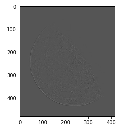
img_mask = (img - cv2.filter2D(img, -1, kernel)) * 9
img_mask = (img_mask - img_mask.mean()) / (img_mask.max() - img_mask.min())
fig, ax = plt.subplots(1, 1)
ax.imshow(img_mask, cmap=‘gray‘)
plt.show()
最后再说说如何用一阶导数提取细节.
定义
注: 也常常用\(M(x, y) = |\frac{\partial f}{\partial x}| + |\frac{\partial f}{\partial y}|\)代替.
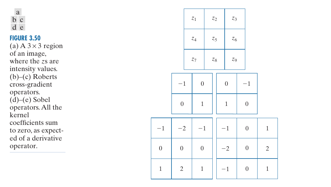
把目标区域按照图(a)区分, Roberts cross-gradient采用如下方式定义:
即右下角的对角之差. 所以相应的kernel变如图(b, c)所示(其余部分为0, \(3 \times 3\)).
注: 计算\(M\)需要两个kernel做两次卷积.
Sobel operators 则是
即如图(d, e)所示.
kernel = np.zeros((3, 3))
kernel[1, 1] = -1
kernel[2, 2] = 1
part1 = cv2.filter2D(img, -1, kernel)
kernel = np.zeros((3, 3))
kernel[1, 2] = -1
kernel[2, 1] = 1
part2 = cv2.filter2D(img, -1, kernel)
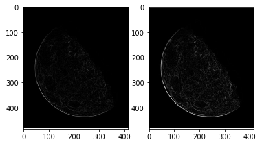
img_roberts = np.sqrt(part1 ** 2 + part2 ** 2)
part1 = cv2.Sobel(img, -1, dx=1, dy=0, ksize=3)
part2 = cv2.Sobel(img, -1, dx=0, dy=1, ksize=3)
img_sobel = np.sqrt(part1 ** 2 + part2 ** 2)
fig, axes = plt.subplots(1, 2)
axes[0].imshow(img_roberts, cmap=‘gray‘)
axes[1].imshow(img_sobel, cmap=‘gray‘)
SHARPENING (HIGHPASS) SPATIAL FILTERS
标签:blur skin digital http contain 算子 load one 差分
原文地址:https://www.cnblogs.com/MTandHJ/p/14890783.html